Attention Residuals (AttnRes) replace the fixed additions in a residual stream with a learned, softmax-weighted mixture of earlier sublayer outputs. This lets each layer select which earlier representations should contribute to its input.

This is attention across model depth rather than across token positions. The regular sequence mechanism, such as Kimi Delta Attention or MLA, still handles interactions between tokens.

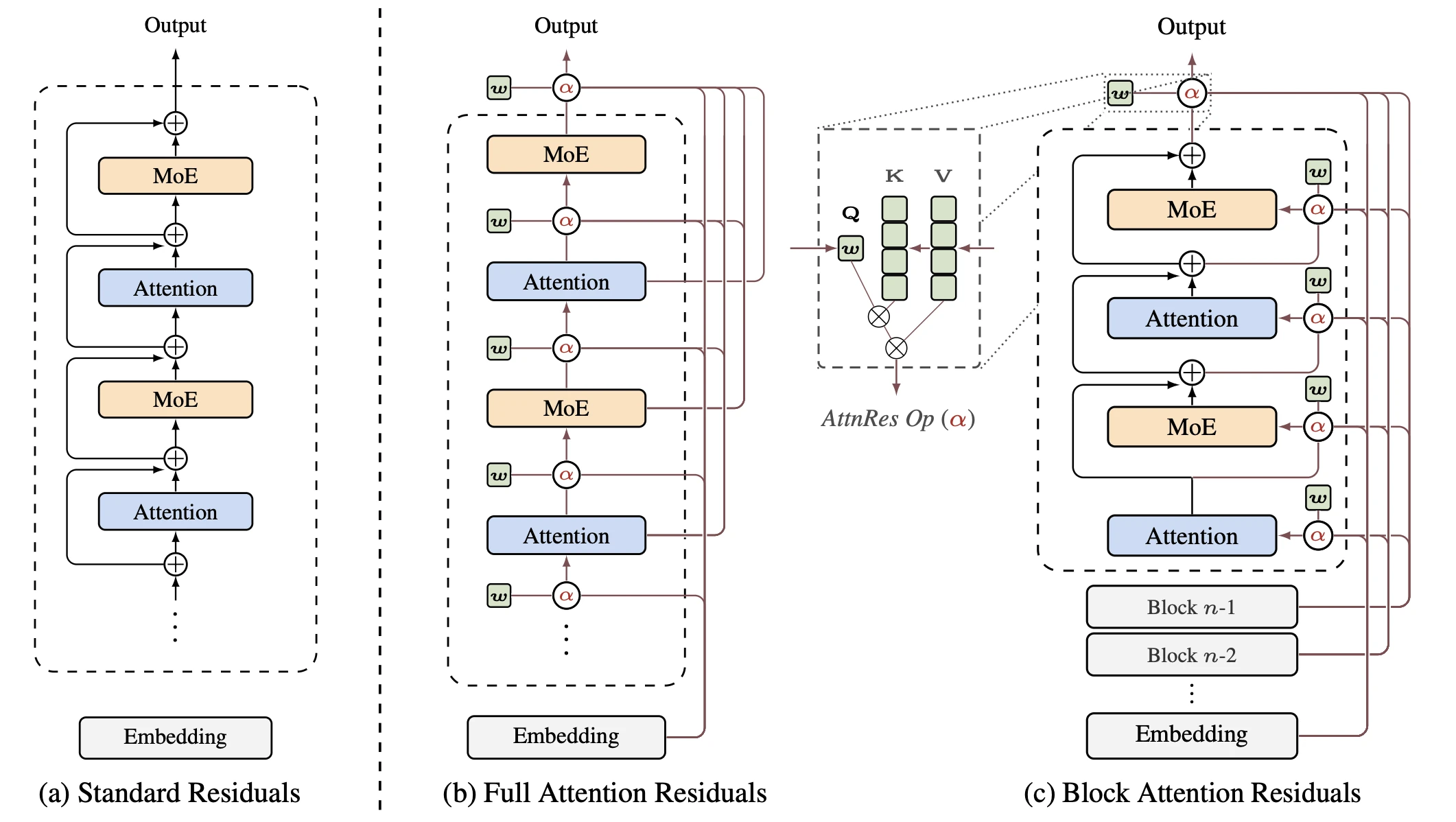
Standard residuals compared with Full and Block Attention Residuals
Standard residuals (left) add every preceding update with a fixed weight of 1. Full AttnRes (center) learns weights over all preceding outputs. Block AttnRes (right) keeps regular additions within blocks and attends over the smaller set of block representations (Original figure source Moonshot AI Attention Residuals repository).

What changes

Fixed residual addition becomes learned softmax weighting over depth

Scalable variant

Block AttnRes attends over block-level representations instead of every sublayer output

Example architectures

Kimi Linear 48B-A3B research variant
Kimi K3

From addition to attention over depth

In a standard PreNorm transformer (like GPT-2 and most others), the input to layer \(l\) is the sum of the embedding and all earlier sublayer outputs:

\[h_l = \sum_{i=0}^{l-1} v_i\]

Here,

  • \(h_l\) denotes the residual-stream representation used as input to sublayer \(l\).
  • \(v_0\) denotes the initial embedding representation, while each \(v_i\) for \(i > 0\) is the update produced by an earlier attention or feed-forward sublayer.

In the standard mechanism above, the embedding and every earlier sublayer output are added with the same weight of 1. AttnRes instead learns how much weight to assign to each one:

\[h_l = \sum_{i=0}^{l-1} \alpha_{i \rightarrow l} \cdot v_i\]

The earlier outputs \(v_i\) serve as values, while their normalized versions \(\phi(v_i)\) serve as keys. For destination layer \(l\), \(w_l\) is the learned pseudo-query vector. It is used to compute the attention weights:

\[\alpha_{i \rightarrow l} = \operatorname{softmax}_i\left(w_l^\top \phi(v_i)\right)\]

The pseudo-query \(w_l\) is a learned model parameter. Each \(\alpha_{i \rightarrow l}\) is the resulting scalar weight for source \(i\). The query is shared across tokens for a given destination layer, but the keys depend on the current token’s earlier representations. The resulting \(\alpha\) weights can therefore differ across tokens.

The pseudo-queries are initialized to zero. This starts the model with uniform depth-wise weights and lets it learn more selective routing during training.

Intuition for the two attention operations

Attention Residuals leave the ordinary self-attention mechanism in place. A transformer using AttnRes performs two separate weighting operations along different axes:

  • Regular self-attention computes weights such as \(A = \operatorname{softmax}(QK^\top)\) between token positions inside an attention sublayer. It mixes information across the sequence.
  • Attention Residuals compute \(\alpha_{i \rightarrow l}\) over earlier attention and feed-forward outputs for the same token. They mix information across model depth to form the next sublayer input \(h_l\).

The \(\alpha\) weights replace the fixed coefficient of 1 used by standard residual accumulation. They do not create another residual branch. After AttnRes constructs \(h_l\), the regular PreNorm attention or feed-forward sublayer consumes it and produces the next update \(v_l\):

earlier sublayer outputs
        ↓  AttnRes mixes across depth using α
next sublayer input h_l
        ↓  regular self-attention or feed-forward layer
new sublayer update v_l

How Attention Residuals and mHC differ

Both methods change the residual path, but along different axes.

Attention Residuals look backward along model depth. For each destination sublayer, they compute one weighted mixture of the embedding and earlier sublayer outputs. Intuitively, the next sublayer can choose which earlier updates to reuse.

mHC widens the residual path into several parallel streams that move forward together. Learned, constrained mappings combine these streams before a sublayer and distribute its output back afterward. Intuitively, the model carries several information lanes through the network and controls how information moves between them.

  • Attention Residuals: select and combine outputs from earlier depths.
  • mHC: maintain and mix several residual streams at the current depth.

With Full Attention Residuals, the number of available earlier outputs grows with model depth. With mHC, the number of parallel streams is fixed, such as the four streams used in DeepSeek V4.

PyTorch-style pseudocode for Full AttnRes

The following side-by-side pseudocode shows where each residual mechanism is used inside a PreNorm transformer block. In both blocks, attention and the MLP receive normalized inputs and compute their updates in the same way. The difference is how each sublayer input is assembled and how its update is carried forward.

Standard residuals

import torch.nn as nn


class StandardTransformerBlock(nn.Module):
    def forward(self, hidden_states):
        # Attention receives the current
        # residual-stream representation.
        attention_update = self.attn(
            self.attn_norm(hidden_states)
        )

        # Add the attention update directly.
        hidden_states = (
            hidden_states + attention_update
        )

        # The MLP sees the residual stream
        # after the attention update.
        mlp_update = self.mlp(
            self.mlp_norm(hidden_states)
        )

        # Add the MLP update directly.
        hidden_states = hidden_states + mlp_update
        return hidden_states

Full Attention Residuals

import torch.nn as nn


class FullAttentionResidualBlock(nn.Module):
    def forward(
        self,
        sources,
        attention_idx,
        mlp_idx,
    ):
        # Build the attention input from the
        # embedding and all earlier updates.
        hidden_states = self.residual_mixer(
            sources, attention_idx
        )

        attention_update = self.attn(
            self.attn_norm(hidden_states)
        )

        # Keep the attention update separate
        # for the next depth-wise mixture.
        sources.append(attention_update)

        # Rebuild the MLP input. The mixer now
        # also sees this block's attention update.
        hidden_states = self.residual_mixer(
            sources, mlp_idx
        )

        mlp_update = self.mlp(
            self.mlp_norm(hidden_states)
        )

        # Keep the MLP update separate too.
        sources.append(mlp_update)
        return sources

At the model level, the standard transformer passes one hidden_states tensor from block to block. Full Attention Residuals begins with sources = [token_embeddings] and passes the growing list between blocks. The attention_idx and mlp_idx arguments identify the two destination sublayers and select their learned pseudo-queries.

The residual_mixer used in the right panel is implemented as follows:

import torch
import torch.nn as nn


class FullAttentionResidual(nn.Module):
    def __init__(self, num_sublayers, d_model):
        super().__init__()

        # Each destination sublayer gets a
        # learned query.
        # Zero initialization starts the
        # depth-wise softmax uniformly.
        self.pseudo_queries = nn.Parameter(
            torch.zeros(num_sublayers, d_model)
        )

        # Normalize sources before using them as keys.
        self.key_norms = nn.ModuleList(
            [
                nn.RMSNorm(d_model)
                for _ in range(num_sublayers)
            ]
        )

    def forward(self, sources, destination_idx):
        # Preserve earlier outputs as separate values.
        # Shape: (sources, batch, tokens, channels)
        values = torch.stack(sources, dim=0)

        # Normalized copies act as depth-wise keys.
        # The final mixture uses the
        # unnormalized values.
        keys = self.key_norms[destination_idx](values)

        # Select the learned query for this destination.
        query = self.pseudo_queries[destination_idx]

        # Score every source separately for every token.
        scores = torch.matmul(keys, query)

        # Normalize the scores across model depth.
        weights = torch.softmax(scores, dim=0)

        # Broadcast each weight across the channels.
        weighted_values = weights.unsqueeze(-1) * values

        # Replace the fixed sum with a weighted mixture.
        return weighted_values.sum(dim=0)

With zero-initialized pseudo-queries, every score starts at zero and the softmax assigns equal weight to all available sources. During training, each token produces different keys from its earlier representations. The same learned pseudo-query can therefore produce different depth-wise weights for different tokens.

Why use blocks?

Full AttnRes has to keep every earlier sublayer output available. That becomes expensive in deep models.

Block AttnRes is an efficiency tweak that groups sublayers into a smaller number of blocks. Ordinary residual additions remain inside each block. At a block boundary, the model keeps one accumulated representation. Later AttnRes operations attend over those completed block representations and the current partial block.

If a model has \(L\) sublayers grouped into \(N\) blocks, the stored depth-wise representations shrink from \(O(Ld)\) to \(O(Nd)\) per token. The paper uses about eight blocks in its large-scale experiments and reports that this retains most of the gain from Full AttnRes.

Compute and memory trade-offs

Attention Residuals add work to the residual path. A standard residual connection only adds vectors. Full AttnRes also normalizes earlier outputs, computes attention scores and a softmax, and forms a weighted sum.

The additional parameter count is negligible because each layer adds only one RMSNorm and one pseudo-query vector. The main costs are the extra attention arithmetic, memory traffic, and communication. With the paper’s optimized implementation, the measured end-to-end training overhead is below 4% with pipeline parallelism, and the inference latency overhead is below 2% on the tested workloads.

Experiments

All experiments in the Attention Residuals paper use the Kimi Linear backbone. The smaller runs isolate the Attention Residuals mechanism across model sizes and ablations. The final run tests Block Attention Residuals in the full 48B-parameter Kimi Linear configuration with 3B active parameters.

Kimi Linear 48B-A3B architecture with Kimi Delta Attention, MLA, and sparse MoE layers
The Kimi Linear 48B-A3B architecture from the gallery. It uses 20 Kimi Delta Attention layers and seven MLA layers arranged in a 3:1 pattern. The full-scale Attention Residuals experiment keeps this backbone and changes the residual connections.

Smaller-scale Attention Residuals experiments from the original Attention Residuals paper

The scaling-law study uses five smaller Kimi Linear models with 194M to 528M active parameters. At each size, it compares a standard PreNorm baseline, Full AttnRes, and Block AttnRes using the same hyperparameters and compute budget. Full and Block AttnRes both reduce validation loss across the five sizes. Based on the fitted scaling curves, Block AttnRes reaches the same loss as a baseline trained with about 1.25 times as much compute.

The separate 16-layer ablation tests which parts of AttnRes produce the improvement. It compares AttnRes with PreNorm, DenseFormer, and mHC, then varies the query, weighting function, normalization, block size, sliding window, and number of heads.

Attention Residuals ablation table and block-size validation-loss plot
The smaller 16-layer ablation compares residual mechanisms and AttnRes design choices. The plot varies the block size from Full AttnRes at one layer per block to increasingly coarse blocks. These are scaled-down experiments, separate from the final 48B Kimi Linear comparison (Original source Attention Residuals).

Full-scale 48B Kimi Linear experiment

The large-scale experiment compares two 48B-parameter Kimi Linear models, each with 3B active parameters. The baseline model keeps the standard PreNorm residual connections. The second model replaces them with Block Attention Residuals. Both models use the same 3:1 Kimi Delta Attention and MLA pattern, MoE structure, depth, hidden dimensions, and training setup. This makes it a controlled comparison of the two residual mechanisms at the full Kimi Linear scale.

Both models were pretrained from scratch on 1.4 trillion tokens. The first 1 trillion tokens are used for the main pretraining phase, followed by about 400 billion higher-quality tokens during mid-training.

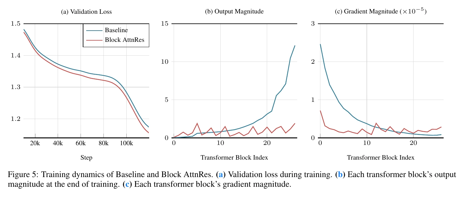
Training dynamics for the 48B Kimi Linear baseline and Block Attention Residuals model
Training dynamics for the full 48B/3B Kimi Linear comparison over the first 1 trillion tokens. Block AttnRes has lower validation loss, bounded blockwise output magnitudes, and more uniform gradient magnitudes (Original source Attention Residuals).

After the complete 1.4-trillion-token recipe, the Block AttnRes model matches or outperforms the standard-residual baseline on every reported downstream benchmark.
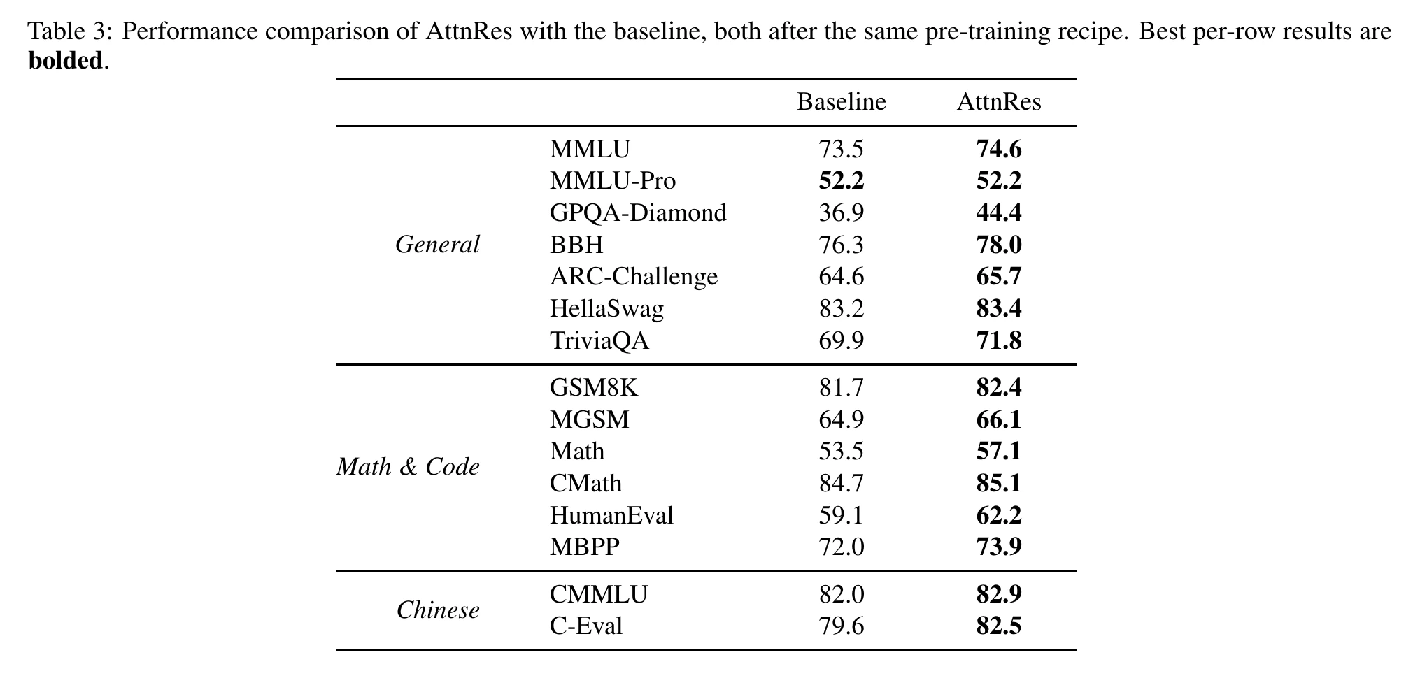
Table comparing benchmark scores for the Kimi Linear baseline and Attention Residuals model
Downstream benchmark comparison between the same full-scale Kimi Linear models after the complete pretraining recipe. The Block Attention Residuals model matches or exceeds the standard-residual baseline on every reported task (Original source Attention Residuals).

Sources