
How does next-token prediction train a large language model?
Next-token prediction trains a large language model by asking it to assign a high probability to the token that actually follows each position in a text sequence. The text supplies both the inputs and the targets, so this training setup is called self-supervised learning. Human annotators do not have to label the next token.
A token is not necessarily a complete word. Depending on the tokenizer, it can represent a word, part of a word, punctuation, or whitespace. The model operates on these token IDs rather than directly on the original text.
Suppose a tokenized chunk contains five tokens. The data loader shifts this sequence by one position:
[
\begin{aligned}
\text{tokens} &= [t_0, t_1, t_2, t_3, t_4]
\text{input} &= [t_0, t_1, t_2, t_3]
\text{target} &= [t_1, t_2, t_3, t_4].
\end{aligned}
]
This single chunk provides four training targets. The model output at the first position is evaluated against (t_1), the second against (t_2), and so forth. A sequence with (L+1) source tokens therefore provides (L) next-token predictions. The practical construction of these windows is covered in How are input-target training examples constructed for LLM pretraining?

The target sequence is used by the loss function. It is not supplied to the transformer as a separate answer. The transformer receives the input sequence, and a causal attention mask prevents each position from reading later input positions. When the model predicts (t_3) from the position containing (t_2), its representation can depend on (t_0), (t_1), and (t_2), but it cannot use (t_3).
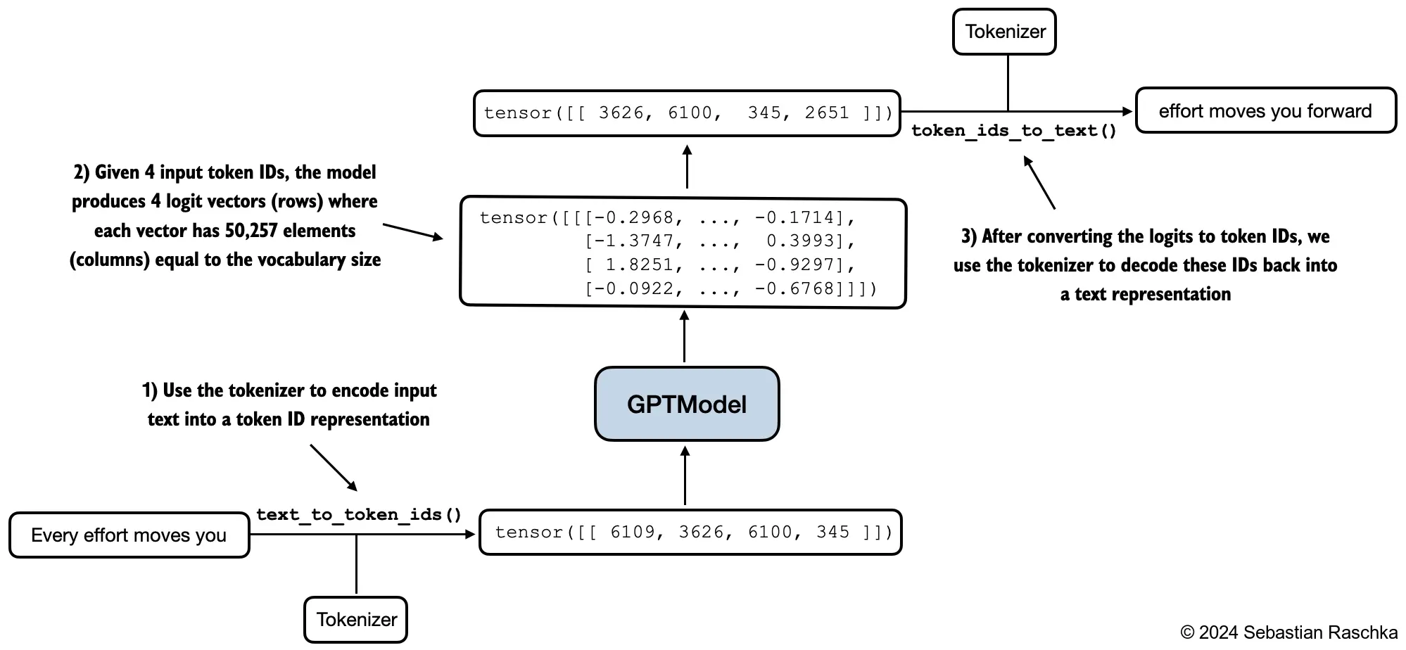
For a batch size (B), sequence length (L), and vocabulary size (V), the model returns a logits tensor with shape
[ B \times L \times V. ]
Each of the (L) positions has one score for every vocabulary entry. Softmax turns these logits into a probability distribution, although training implementations usually pass the raw logits directly to a cross-entropy function that applies the required log-softmax internally.
For a sequence (x_0, x_1, \ldots, x_T), the average next-token loss can be written as
[ \mathcal{L} = -\frac{1}{N} \sum_{i \in \mathcal{I}} \log p_\theta(x_i \mid x_{<i}), ]
where (\mathcal{I}) contains the (N) valid target positions. If the model assigns probability 0.5 to the correct token, that position contributes about 0.693 to the loss. A probability of 0.01 contributes about 4.605. Assigning little probability to the observed continuation is therefore penalized strongly.
Padding tokens are normally excluded from (\mathcal{I}). During instruction finetuning, a training recipe may also exclude user-prompt or template positions so the loss focuses on the assistant response. The same basic next-token objective still applies to every included position.

Backpropagation differentiates this average loss through the output layer and the transformer. The optimizer then updates the token embeddings, attention layers, feed-forward layers, normalization parameters, and output projection. Repeating this process across many batches makes continuations found in similar contexts more probable.
During training, the complete text chunk is already known. This allows the model to score all (L) positions in one masked forward pass, a setup commonly called teacher forcing. The causal mask prevents future-token leakage even though the matrix operations for the positions run together. Why is inference sequential while training is much more parallel? discusses this distinction in more detail.
Generation uses the same learned conditional probabilities in a different loop. The model processes the current context, selects a token from the final logits, appends that token, and runs the next decoding step. The continuation is unknown, so future decoding steps cannot be computed in advance. See How does autoregressive text generation work at inference time? for the complete loop.
Next-token prediction teaches a base model to approximate patterns in its training text. It does not directly provide labels for factual correctness, helpfulness, or instruction following. Those properties depend on the data, model capacity, and later training stages. The pretraining objective itself remains the concrete probabilistic task of increasing the likelihood of the observed next tokens across the corpus.