How does autoregressive text generation work at inference time?
At inference time, autoregressive text generation works by repeatedly predicting one new token from the current context, appending that token to the sequence, and then running the model again on the updated sequence.
This is called autoregressive because the model conditions each new prediction on the tokens that came before, including the tokens it generated itself in earlier steps.
The loop is conceptually simple:
- Start with a prompt.
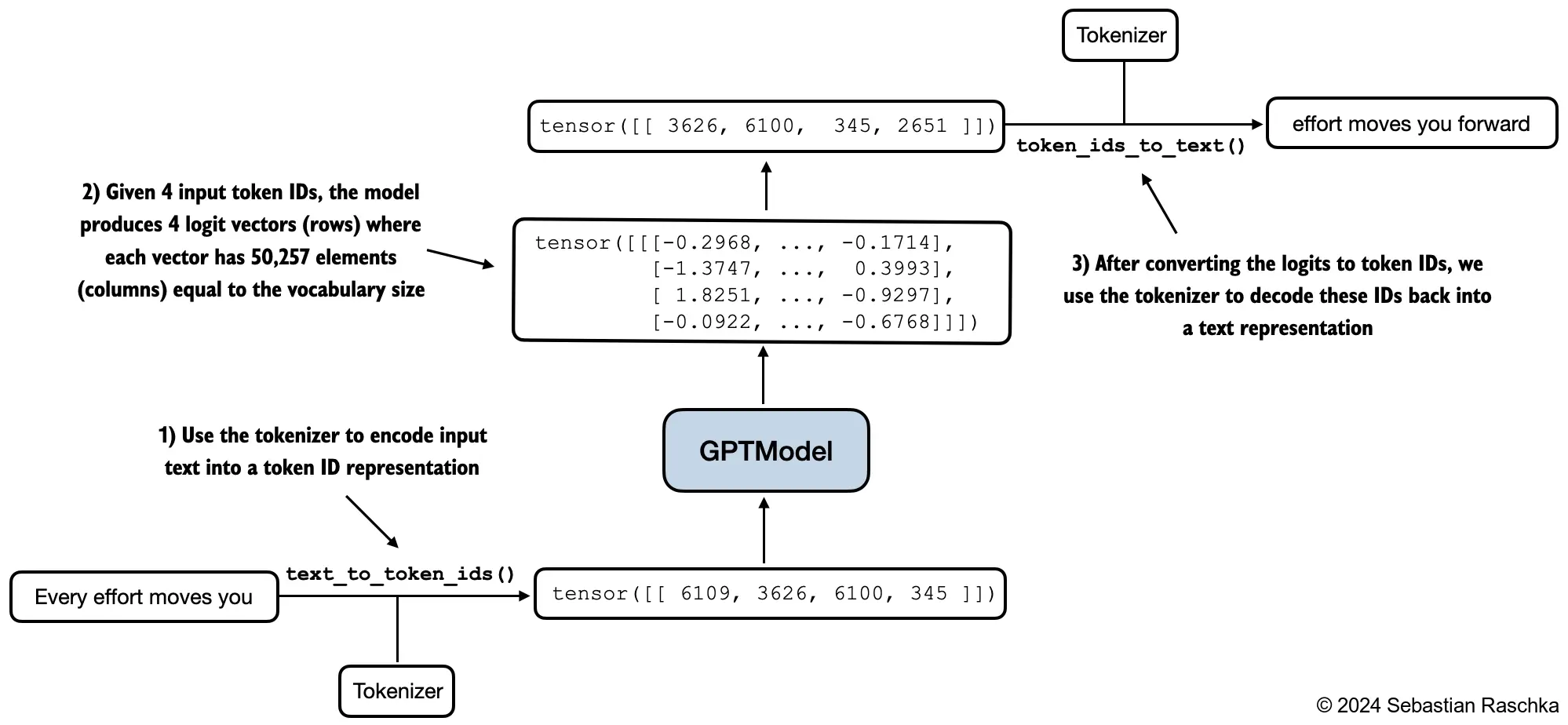
- Tokenize it and feed it into the model.
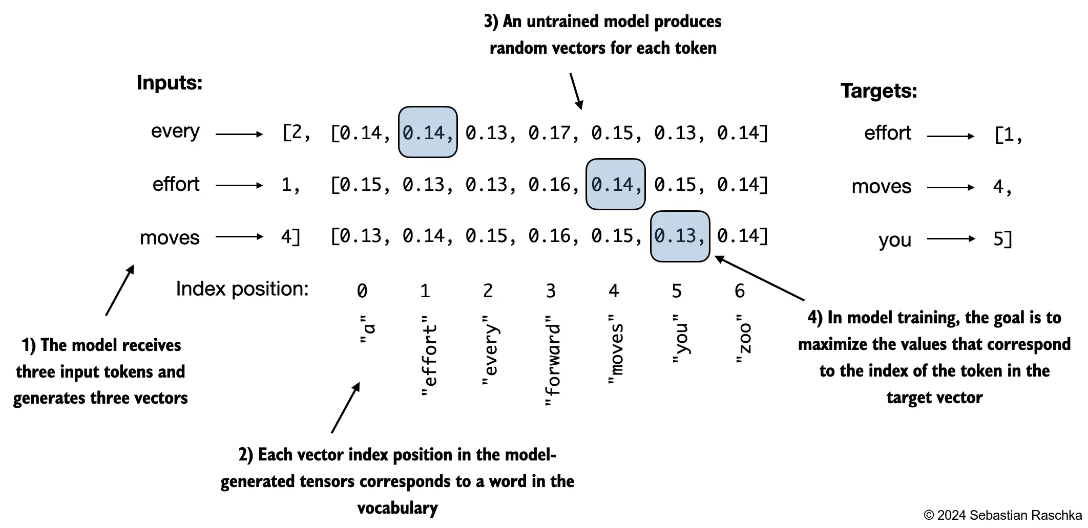
- Read the logits for the last position.
- Convert those logits into a probability distribution over the vocabulary.
- Choose the next token, for example with greedy decoding or sampling.
- Append that token to the running sequence.
- Repeat until a stop condition is reached.
The key detail is that, although the model produces one logits vector for every input position, only the last position is used to pick the next token during generation. The earlier positions correspond to earlier prediction tasks that were already resolved by the current prefix.
Once the model produces logits for that last position, those scores are turned into probabilities. Then a decoding rule decides which token to emit:
- Greedy decoding chooses the highest-probability token.
- Sampling draws from the distribution, often with temperature or top-k constraints.
The selected token ID is then decoded later back into text.
Then the whole process repeats on the extended prefix. If the prompt was “Every effort moves you” and the next token chosen is a comma, the next model call conditions on “Every effort moves you,” and then predicts the token after that comma, and so on.
This explains both the power and the cost of LLM inference:
- It is powerful because each token can depend on the full generated prefix.
- It is expensive because generation is inherently sequential across output tokens.
Training is more parallel: the model can compute losses for many token positions in one pass. Inference is less parallel because token t+1 cannot be chosen until token t has already been generated.
In practice, real systems add optimizations such as a KV cache so the model does not recompute everything from scratch at every step. But the high-level generation logic stays the same.
The process stops when one of several conditions is met:
- the model emits a stop or end-of-text token
- it reaches a maximum number of new tokens
- an application-level stopping rule is triggered
In short, autoregressive generation is a repeated next-token prediction loop: the model predicts one token from the current prefix, appends it, and uses the longer prefix to predict the next one.