Losses Learned
-- Optimizing Negative Log-Likelihood and Cross-Entropy in PyTorch (Part 1)
The cross-entropy loss is our go-to loss for training deep learning-based classifiers. In this article, I am giving you a quick tour of how we usually compute the cross-entropy loss and how we compute it in PyTorch. There are two parts to it, and here we will look at a binary classification context first.
You may wonder why bother writing this article; computing the cross-entropy loss should be relatively straightforward!? Yes and no. We can compute the cross-entropy loss in one line of code, but there’s a common gotcha due to numerical optimizations under the hood. (And yes, when I am not careful, I sometimes make this mistake, too.) So, in this article, let me tell you a bit about deep learning jargon, improving numerical performance, and what could go wrong.
Pop quiz
Let’s start this article with a little quiz. Assume we are interested in implementing a deep neural network classifier in PyTorch. The code is as follows:
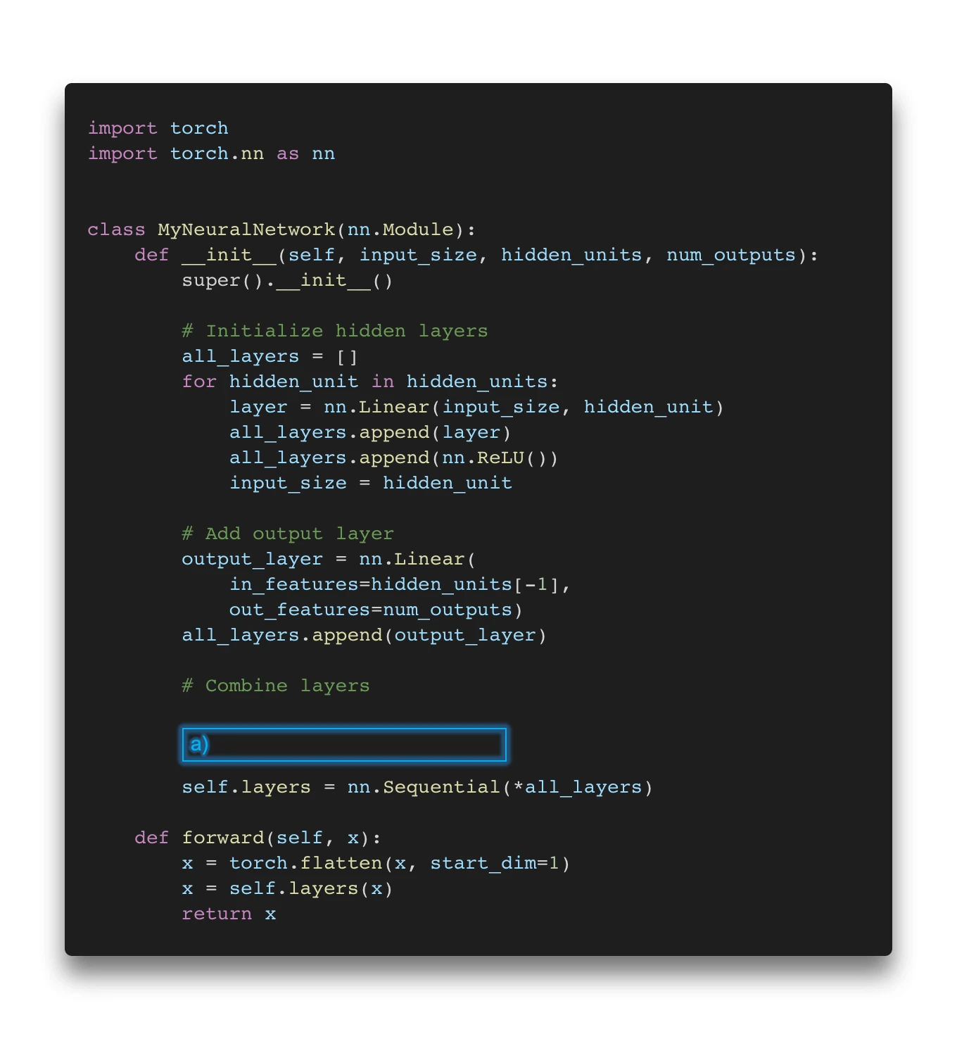
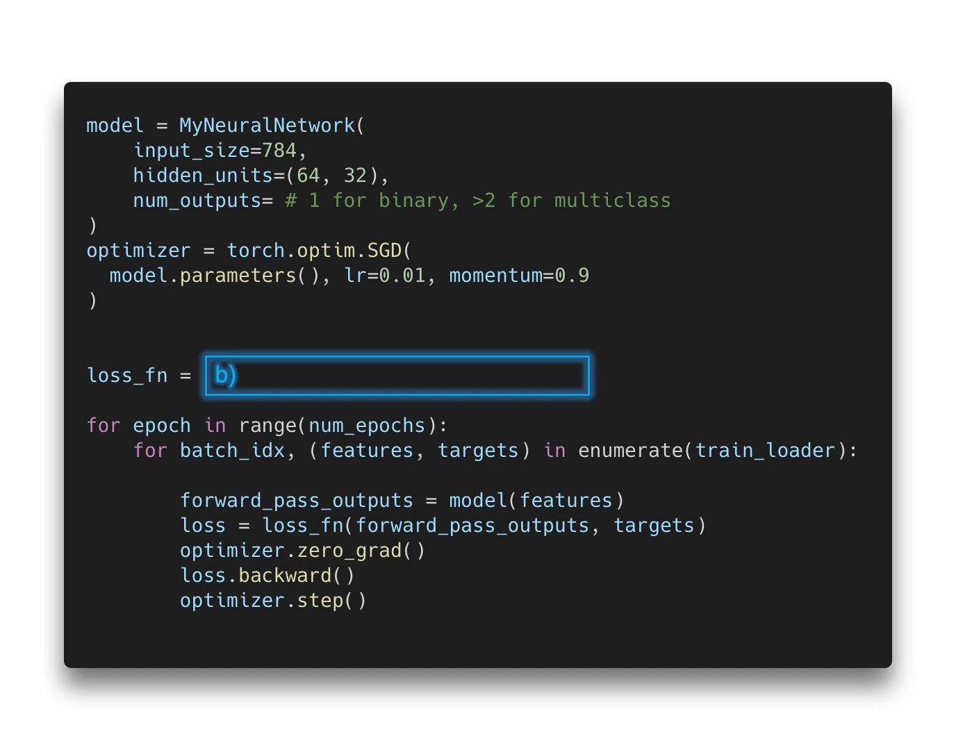
Oh no, two essential parts are missing! Now, there are several options to fill in the missing code for the boxes (a) and (b), where blank means that no additional code is required.
If you are interested in a binary classification task (e.g., predicting whether an email is spam or not), these are some of the options you may choose from:
Binary classification
-
(a) blank & (b)
nn.BCELoss() -
(a) blank & (b)
nn.BCEWithLogitsLoss() -
(a)
nn.Sigmoid& (b)nn.BCELoss() -
(a)
nn.Sigmoid& (b)nn.BCEWithLogitsLoss() -
(a)
nn.LogSigmoid& (b)nn.BCELoss() -
(a)
nn.LogSigmoid& (b)nn.BCEWithLogitsLoss()
(Note that BCELoss is short for binary-cross entropy loss.)
And here’s the challenge!
Question 1: Which of the six options above is the best approach?
Question 2: Which of these options is/are acceptable but not ideal?
Question 3: Which options is/are wrong?
Next, let’s repeat this game considering a multiclass setting, like classifying nine different handwritten digits in MNIST. There are the following options:
Multiclass classification
- (a) blank & (b)
nn.NLLLoss() - (a) blank & (b)
nn.CrossEntropyLoss() - (a)
self.layers.append(nn.Softmax())& (b)nn.NLLLoss() - (a)
self.layers.append(nn.Softmax())& (b)nn.CrossEntropyLoss() - (a)
self.layers.append(nn.LogSoftmax())& (b)nn.NLLLoss() - (a)
self.layers.append(nn.LogSoftmax())& (b)nn.CrossEntropyLoss()
(Note that NLLLoss is short for negative log-likelihood loss.)
If you are confident about your answers and can explain them, you probably don’t need to read the rest of the article. However, if you are unsure, I encourage you to continue reading.
The binary cross-entropy loss
The quiz in the previous section introduced two losses, the NLLLoss (short for negative log-likelihood loss) and the CrossEntropyLoss. Conceptually, the negative-log likelihood and the cross-entropy losses are the same. To understand the relationship between those and see how these concepts connect, let’s take a step back and start with a binary classification problem. Here binary means that the classification problem has only two unique class labels (for example, email spam classification with the two possible labels spam and not spam).
Binary classification and the logistic loss function
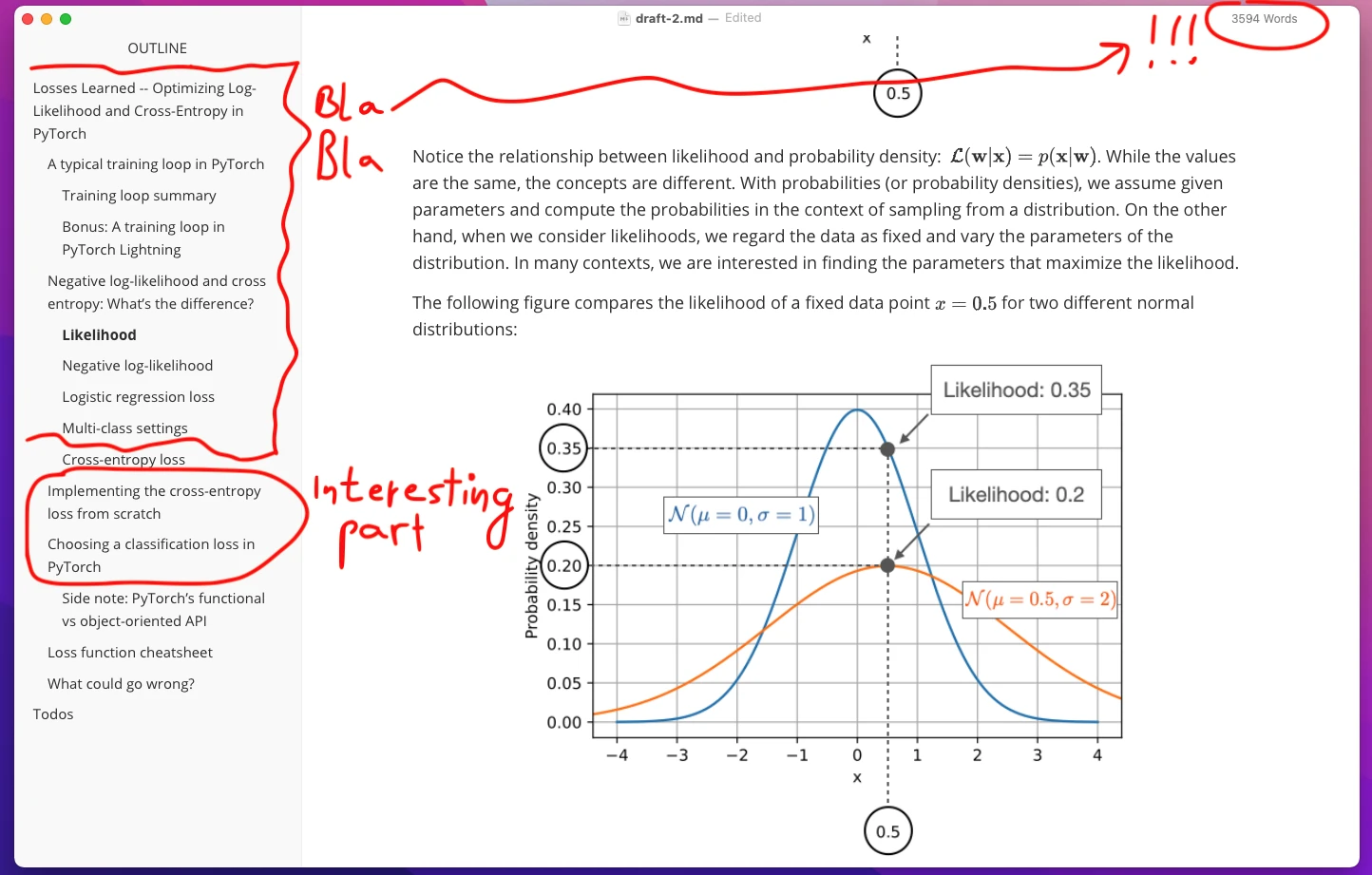
In statistics, we often talk about the concept of maximum likelihood estimation, which is an approach for estimating the parameters of a probability distribution or model. In particular, we are given a data sample, and we want to find the parameters of a model that maximize the likelihood function. Due to numeric advantages, we usually apply a log transformation to the likelihood function. (Since the log function is a monotonically increasing function, the parameters that maximize the likelihood also maximize the log-likelihood.) Also, we like to multiply the log-likelihood by (\(-1\)) such that it becomes a negative log-likelihood. This turns the maximization problem (maximizing the log-likelihood) into a minimization problem (minimizing the negative log-likelihood).
So, to find the optimal parameters, we can maximize the log-likelihood, or we can minimize the negative log-likelihood. If this sounds confusing, think about the classification accuracy and error. If a classifier has \(80\%\) accuracy, its classification error is \(100\% - 80\%= 20\%\). And maximizing accuracy serves the same goal as minimizing the error.
To recap,
-
we have a likelihood function \(\mathcal{L}\left(\mathbf{w} \; \vert \; x^{(1)}, ..., x^{(n)}\right)\), where \(\mathbf{w}\) is a vector of parameters we are trying to optimize given a set of data points \(x^{(1)}, ..., x^{(n)}\).
-
We apply a log transformation and multiplication by \((-1)\), such that we get the negative log-likelihood \(- \log \mathcal{L}\left(\mathbf{w} \; \vert \; x^{(1)}, ..., x^{(n)}\right)\).
Now, the negative log-likelihood can be rewritten as follows:
\[-\log \mathcal{L}\left(\mathbf{w} \; \vert \; x^{(1)}, ..., x^{(n)}\right) = - \sum_{i=1}^{n} \log \mathcal{p}\left(x^{(i)}\vert \mathbf{w}\right),\]where \(\mathcal{p}(x^{(i)}\vert \mathbf{w})\) is a quantity from, for example, a probability density function.
In the context of machine learning and classifiers, we usually also involve class labels \(y^{(1) } ... y^{(n)}\). Considering a logistic regression classifier, we are modeling the class-membership probability \(\mathcal{p}(y^{(i)} \vert \mathbf{x}^{(i)} , \mathbf{w})\) of the \(i\)-th training example given model parameters \(\mathbf{w}\) (to keep the notation simple, please assume the bias unit is part of the weight vector \(\mathbf{w}\)).
So, the negative log-likelihood loss becomes
\[- \log \mathcal{L}\left( \mathbf{w} \; \vert \; \mathbf{X}, \mathbf{y}\right) = - \sum_{i=1}^{n} \log \mathcal{p}\left(y^{(i)} \; \vert \; \mathbf{x}^{(i)}; \mathbf{w}\right).\]Skipping a few steps for brevity (some more details in my book 😉), for logistic regression, this expands to the following:
\[- \log \mathcal{L}\left( \mathbf{w} \; \vert \; \mathbf{X}, \mathbf{y}\right) = - \sum_{i=1}^{n}\left[y^{(i)} \log \left(\sigma\left(z^{(i)}\right)\right) + \left(1-y^{(i)}\right) \log \left(1-\sigma\left(z^{(i)}\right)\right)\right].\]The \(z^{(i)}\) in the equation above is used to simplify the notation, where
- \(z^{(i)}\) represents the weight inputs, \(z^{(i)}\ = \mathbf{w}^{\top} \mathbf{x}^{(i)} + b\), which are also often called logits. (And \(b\) is the bias unit, which we omitted previously to keep the notation simpler.)
- \(\sigma(\cdot)\) is the logistic sigmoid function, \(\sigma(z) = 1 / (1 + e^{-z}).\)
In practice, we also call this equation above the logistic loss function or binary cross-entropy. To summarize, the so-called logistic loss function is the negative log-likelihood of a logistic regression model. And minimizing the negative log-likelihood is the same as minimizing the cross-entropy. How the cross-entropy is derived is a story for another time.
In addition, we also often add a scaling factor \(\frac{1}{n}\), to average over the training set size or batch size and write it as a function of the weighted inputs \(\mathbf{Z}\) and corresponding labels \(\mathbf{y}\):
\[L_\mathbf{w}\left( \mathbf{y} , \mathbf{Z} \right) = - \frac{1}{n} \sum_{i=1}^{n}\left[y^{(i)} \log \left(\sigma\left(z^{(i)}\right)\right) + \left(1-y^{(i)}\right) \log \left(1-\sigma\left(z^{(i)}\right)\right)\right].\]By the way, we usually use the same loss function for any type of multilayer neural networks for binary classification. We use the logistic sigmoid function \(\sigma(\cdot)\) in the output layer, and the logits $z$ are the weighted inputs at the output layer as illustrated in the figure below:
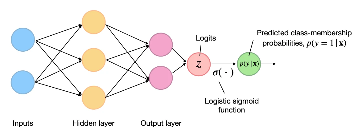
(Note that the superscript indices in the figure above are indexing the layers, not training examples.)
Implementing the binary cross-entropy loss from scratch
(You can find a Jupyter notebook containing the following code snippets here.)
The previous section illustrated the origins of the negative log-likelihood loss, which is synonymous to the logistic loss and binary cross-entropy loss in a binary classification context.
In this section, we will implement the logistic loss function for binary classification settings – these are scenarios where we have two class labels, 0 and 1. Implementing concepts from scratch is my favorite way of solidifying my understanding.
But before we get started, did you notice that the logistic loss,
\[L_\mathbf{w}\left( \mathbf{y} , \mathbf{Z} \right) = - \frac{1}{n} \sum_{i=1}^{n}\left[y^{(i)} \log \left(\sigma\left(z^{(i)}\right)\right) + \left(1-y^{(i)}\right) \log \left(1-\sigma\left(z^{(i)}\right)\right)\right],\]consists of two parts? Namely,
Part 1: \(y^{(i)} \log \left(\sigma\left(z^{(i)}\right)\right),\) and
Part 2: \(\left(1-y^{(i)}\right) \log \left(1-\sigma\left(z^{(i)}\right)\right)\).
If \(y^{(i)}=0\), then the portion on the left, \(y^{(i)} \log \left(\sigma\left(z^{(i)}\right)\right)\) cancels because \(0\times\) something is \(0\). Vice versa, if \(y^{(i)}=1\), then the second expression, \(\left(1-y^{(i)}\right) \log \left(1-\sigma\left(z^{(i)}\right)\right)\) cancels because \(\left(1-y^{(i)}\right)=(1-1)=0\).
This will allow us to implement the logistic loss (which we will call binary cross-entropy from now on) from scratch by using a Python for-loop (for the sum) and if-else statements. Personally, when I try to implement a new concept, I often opt for naive implementations before optimizing things, for example, using linear algebra concepts. This often helps me understand things better, making the code easier to debug (for me).
So, to illustrate the concept of the binary cross-entropy loss above, let’s define a small toy dataset consisting of five training examples. And we have an arbitrary neural network classifier with one output node, as shown below:
Or, to make it more concrete, consider a multilayer perceptron (as shown in the figure above) implemented in PyTorch:
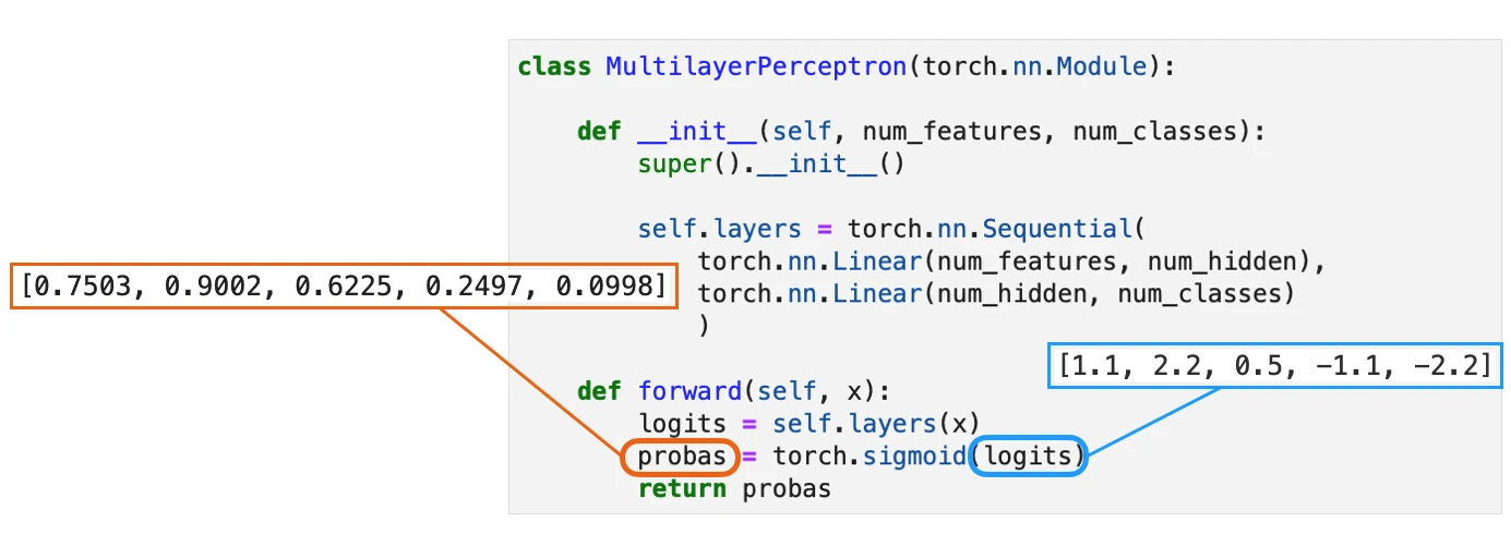
We assume that we fed this network a batch of five training examples for which it returned five outputs, as shown in the figure above. To keep the code examples more minimalist, we skip this step and hard-code the neural network outputs – the logits and probas – as shown below:
In:
import torch


y_targets = torch.tensor([1., 1., 0., 0., 0.])

logits = torch.tensor([1.1, 2.2, 0.5, -1.1, -2.2])
probas = torch.sigmoid(logits)
print(probas)
Out:
tensor([0.7503, 0.9002, 0.6225, 0.2497, 0.0998])
Now, after all this setup, let’s get to the from-scratch implementation – a naive version using Python for-loops as promised above:
In:
def binary_logistic_loss_v1(probas, y_targets):
    res = 0.
    for i in range(y_targets.shape[0]):
        if y_targets[i] == 1.:
            res += torch.log(probas[i])
        elif y_targets[i] == 0.:
            res += torch.log(1-probas[i])
        else:
            raise ValueError(f'Value {y_targets[i]} not allowed')
    res *= -1
    res /= y_targets.shape[0]

    return res


binary_logistic_loss_v1(probas, y_targets)
Out:
tensor(0.3518)
In the code implementation above, we iterated ofter the training examples and then computed the loss using one of the two parts, dependent on the class label, that we defined earlier.
Part 1: \(y^{(i)} \log \left(\sigma\left(z^{(i)}\right)\right),\) and
Part 2: \(\left(1-y^{(i)}\right) \log \left(1-\sigma\left(z^{(i)}\right)\right)\).
We added the loss terms for all \(n\) training examples (where \(n=\)y_targets.shape[0]) and then returned the loss as the average. The Python binary_logistic_loss_v1 function is very verbose, but at the same time, it is very easy to read and easy to reason about. Drafting a function like this is an excellent way to ensure it produces the results we intend.
Improving our from-scratch implementation using concepts from linear algebra
In the previous section, we implemented the binary cross-entropy loss from scratch using Python for-loops. In my experience, this is often a great way to start. In this section, we will now see how we can make this implementation more efficient.
In practice, we can often replace expensive for-loops with concepts from linear algebra. For example, we can implement the previous function using vector dot-products (via PyTorch’s matmul, short for matrix-multiplication):
We assume that we fed this network a batch of five training examples for which it returned five outputs, as shown in the figure above. To keep the code examples more minimalist, we skip this step and hard-code the neural network outputs – the logits and probas – as shown below:
In:
def binary_logistic_loss_v2(probas, y_targets):
    first = -y_targets.matmul(torch.log(probas))
    second = -(1 - y_targets).matmul(torch.log(1 - probas))
    return (first + second) / y_targets.shape[0]

binary_logistic_loss_v2(probas, y_targets)
Out:
tensor(0.3518)
Above, we were able to replace the for loops with dot products. For example,
res = 0.
for i in range(y_targets.shape[0]):
    if y_targets[i] == 1.:
        res += torch.log(probas[i])
becomes
first = -y_targets.matmul(torch.log(probas))
That’s because a dot-product is equivalent to a weighted sum:
\[\mathbf{a}^{\top} \mathbf{b} = \sum_i a_i b_i.\]And as we discussed earlier, for the first term, the cases where \(y=0\) are not affecting the sum due to the multiplication with \(0\) resulting in products that are \(0\). (Equivalently, the second term skips cases with \(y=1\) due via the term \(1 - y\).)
Not only is the binary_logistic_loss_v2 function more compact than _v1, it is also faster. You could try to run the following %timeit lines of code in a Jupyter notebook and see for yourself:
In:
%timeit binary_logistic_loss_v1(probas, y_targets)
Out:
38 µs ± 286 ns per loop (mean ± std. dev. of 7 runs, 10,000 loops each)
In my case, even with the small 5-element input vectors, _v2 runs about \(5\times\) faster (10.6 µs) than _v1 (38 µs) on my laptop:
In:
%timeit binary_logistic_loss_v2(probas, y_targets)
Out:
10.6 µs ± 81.9 ns per loop (mean ± std. dev. of 7 runs, 100,000 loops each)
While implementing a loss function from scratch is a great learning exercise, we usually want to use efficient implementations from established deep learning libraries for real-world applications. The from-scratch implementation served the purpose that we can show the logistic loss (which we implemented as binary_logistic_loss_v) produces the same results as the binary cross-entropy implementations in PyTorch, which we will cover in the same section. This gives us confidence that we understand the binary cross-entropy formula and that it is indeed the same concept as the logistic loss or negative log-likelihood.
Using the binary cross-entropy loss in PyTorch
Now, let’s see how we can implement the binary cross-entropy loss in PyTorch. The common way is to use the loss classes from torch.nn:
In:
bce = torch.nn.BCELoss()
bce(probas, y_targets)
Out:
tensor(0.3518)
(In a later section, we will see that there are also “functional” version in torch.nn.functional.)
As we can see from the code output above, the PyTorch BCELoss produces exactly the same results as our own binary_logistic_loss_v functions. Yay!
Using the object-oriented API, we first instantiated the loss via BCELoss, and then we used used it like a function. This works because the BCELoss and other losses in PyTorch have and has an underlying forward() method that is executed when calling bce(...).
Under the hood, we can picture it as something like this:
In:
class MyBCELoss(torch.nn.Module):
    def __init__(self):
        super().__init__()

    def forward(self, inputs, targets):
        return binary_logistic_loss_v2(inputs, targets)


my_bce = MyBCELoss()
my_bce(probas, y_targets)
Out:
tensor(0.3518)
Why are there two binary cross-entropy losses in PyTorch?
Before we move on and extend the binary cross-entropy loss to a multiclass setting, one more thing is worth mentioning. When we used BCELoss, the inputs were the class membership probabilities (probas) similar to our own binary_cross_entropy_v functions. Interestingly, there is a second binary cross-entropy loss implementation, namely, BCELossWithLogits:
In:
bce_logits = torch.nn.BCEWithLogitsLoss()
bce_logits(logits, y_targets)
Out:
tensor(0.3518)
As we can see, the results are still the same. The difference here is that BCELossWithLogits accepts the logits (weighted inputs of the output layer) instead of the class-membership probabilities. Instead of us having to pass the logits through a logistic sigmoid function,
In:
bce = torch.nn.BCELoss()
bce(torch.sigmoid(logits), y_targets)
Out:
tensor(0.3518)
the BCEWithLogitsLoss applies the sigmoid function internally.
So, why does PyTorch implement two versions of the binary cross-entropy loss, and which one should we use? I guess it implements the BCELoss because it’s the canonical form, which is what most people are familiar with. However, in practice, I highly urge you to consider using the BCEWithLogitsLoss if you are working with the binary cross-entropy (in the next part, we will also see how we can use the regular CrossEntropyLoss) for binary classification.
The reason why we want to use BCEWithLogitsLoss is improved numerical stability due to the log-sum-exp trick. (You can find the source code implementation here.) In general, another important concept when using PyTorch (or any deep learning library, really) is to make use of fused operators. One example is the logsigmoid(z) function that we can use instead of log(sigmoid(z)) – operator fusing makes code run much faster, especially on the GPU.
Recall our own binary cross-entropy loss implementation, which is shown again below:
In:
def binary_logistic_loss_v2(probas, y_targets):
    first = -y_targets.matmul(torch.log(probas))
    second = -(1 - y_targets).matmul(torch.log(1 - probas))
    return (first + second) / y_targets.shape[0]

binary_logistic_loss_v2(probas, y_targets)
Out:
tensor(0.3518)
We can replace torch.log(probas) by torch.nn.functional.logsigmoid(logits) as follows:
In:
import torch.nn.functional as F


def binary_logistic_loss_v3(logits, y_targets):
    first = -y_targets.matmul(F.logsigmoid(logits))
    second = -(1 - y_targets).matmul(F.logsigmoid(logits) - logits)
    return (first + second) / y_targets.shape[0]

binary_logistic_loss_v3(logits, y_targets)
Out:
tensor(0.3518)
(By the way, I have no idea why torch.sigmoid is not under torch.nn.functional like logsigmoid.)
Why the replacement in first = ... was pretty straightforward, you may wonder what happened in second = ... , that is, why torch.log(1 - probas) became F.logsigmoid(logits) - logits). This is allowed because
(By the way, we also use this trick for the CORN loss in Deep Neural Networks for Rank-Consistent Ordinal Regression Based On Conditional Probabilities.)
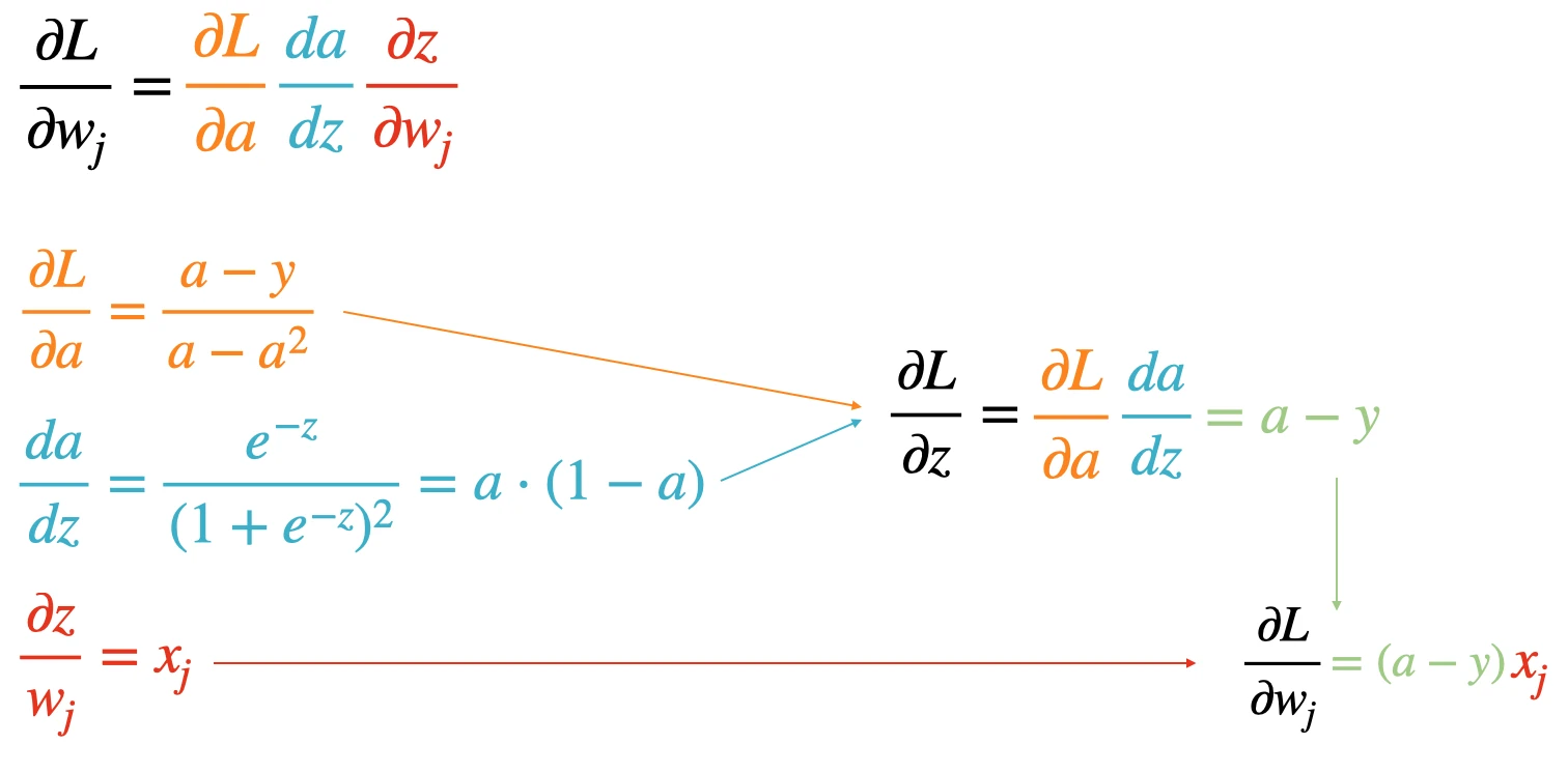
As a sidenote, technically, it is also possible to simplify the backprop pass. But that’s something both version of the loss should already be doing internally.
For instance, instead of having the automatic differentiation engine compute the numerical gradient for the three terms and join them together as follows, \(\frac{\partial L}{\partial w_{j}}= \frac{\partial L}{\partial a} \frac{d a}{d z} \frac{\partial z}{\partial w_{j}} = \frac{a-y}{a-a^{2}} a \cdot (1-a) x_j,\) we could compute the simplified form, \(\frac{\partial L}{\partial w_j} = (a-y) x_j.\) The simplified form should be faster to compute and numerically more stable. We can derive it as illustrated in the figure below:
PyTorch’s two binary-cross entropy implementations in practice
The previous section explained that there are two binary cross-entropy implementations in PyTorch, BCELoss and BCEWithLogitsLoss. We discussed that it is recommended to use BCEWithLogitsLoss over BCELoss due to the log-sum trick for improved numerical stability. To see if this makes any difference in practice, I implemented a VGG-16 convolutional neural network and trained it on CelebA face images to predict whether someone is smiling or not.
It’s worth emphasizing again that the difference is not the computational speed but numerical stability. For instance, the classifier trained with Logits+BCEWithLogitsLoss (vgg16-bcewithlogitsloss.ipynb) reaches ~92% accuracy after 4 epochs, whereas the Sigmoid+BCELoss version (vgg16-bceloss.ipynb) does not even converge with the same hyperparameter settings.
PyTorch’s functional vs object-oriented API
In the previous section, we used PyTorch’s object-oriented implementations of the binary cross-entropy losses. Object-oriented here means that they are implemented as a Python class, and we have to instantiate objects to use those. Object-oriented paradigms are great if we have to keep track of internal states (like model weights and gradients).
However, in case of things that don’t require internal states, like loss functions, we can also use the functional API that saves us from the extra step of having to instantiate the losses. In other words, PyTorch’s functional API, via the torch.nn.functional submodule, offers implementations without an internal state.
The “functional” equivalents of our previously used loss functions are as follows:
Binary cross-entropy
import torch.nn.functional as F

F.binary_cross_entropy(probas, y_targets)
Out:
tensor(0.3518)
Binary cross-entropy with logits
In:
import torch.nn.functional as F

F.binary_cross_entropy_with_logits(logits, y_targets)
Out:
tensor(0.3518)
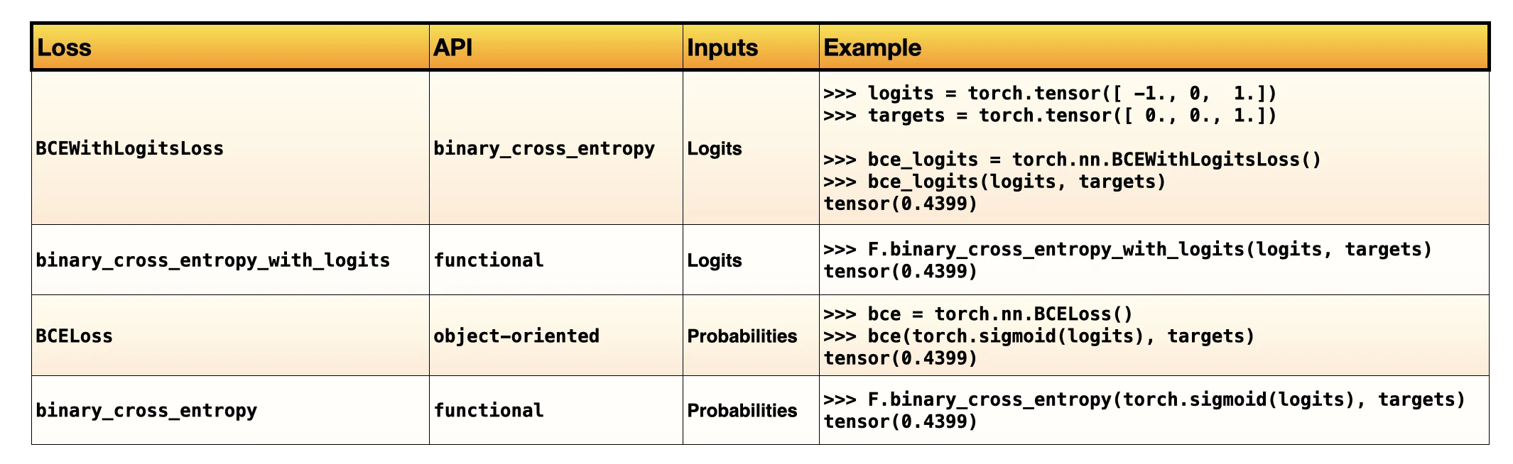
A PyTorch loss function cheatsheet (so far)
Let’s summarize what we have covered so far. There are two binary cross-entropy loss functions in Python – actually, four, if we distinguish between the objected-oriented and functional versions. The table below summarizes the loss functions we covered thus far in this first part of the article:
I hope you are now confident about answering the quiz for the Binary classification part.
What’s next
In the next part, we will extend the concepts from this post and look into the cross-entropy loss for multiple classes. Finally, we will learn about some infamous inconsistencies in the PyTorch API and cover all the remaining bits and pieces for solving the pop quiz 😉.
Thank you for reading. If you liked this article, you can also find me on Twitter, where I share more helpful content.
Outtakes: The missing sections
In my first draft, I ended up writing 3600 words before I even got to the main part I set out to write.
I am not sure if any of you has the endurance to read all of that. Also, there was way too much math and not enough code. Blog posts should be fun!
So, to keep things more succinct, I scrapped all of that and started over. The second time around, I am made a few assumptions:
-
I assumed you already knew what likelihoods are.
-
Also, you were already familiar with the negative log-likelihood loss we minimized when training deep neural networks.
-
And you probably heard that the negative log-likelihood loss and cross-entropy loss are the same thing.
-
You also knew how a typical PyTorch training loop looks like.
-
By the way, I am also assumed that you were familiar with the concept of logits and the softmax activation function.
I am glad we were all on the same page 😊.
Read Next
 Build a Reasoning Model From Scratch Is Out
Short note announcing the release of Build a Reasoning Model From Scratch and linking the publisher and Amazon pages.
Build a Reasoning Model From Scratch Is Out
Short note announcing the release of Build a Reasoning Model From Scratch and linking the publisher and Amazon pages.
 Using Local Coding Agents
Short note linking a new article on setting up local coding agents with open-weight models.
Using Local Coding Agents
Short note linking a new article on setting up local coding agents with open-weight models.
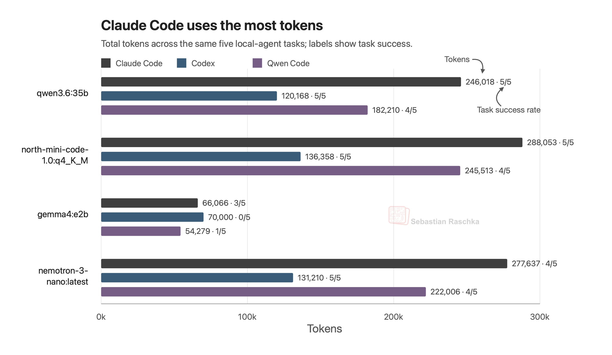 Local Open-Weight LLMs in Coding Harnesses
Short note on trying local open-weight LLMs across Qwen-Code, Codex, and Claude Code harnesses.
Local Open-Weight LLMs in Coding Harnesses
Short note on trying local open-weight LLMs across Qwen-Code, Codex, and Claude Code harnesses.

If you read the book and have a few minutes to spare, I'd really appreciate a brief review. It helps us authors a lot!
Your support means a great deal! Thank you!