Machine Learning FAQ

Negative log-likelihood

The FAQ entry What is the difference between likelihood and probability? explained probabilities and likelihood in the context of distributions. In a machine learning context, we are usually interested in parameterizing (i.e., training or fitting) predictive models. Or, more specifically, when we work with models such as logistic regression or neural networks, we want to find the weight parameter values that maximize the likelihood.

Let’s use the notation \(\mathbf{x}^{(i)}\) to refer to the \(i\)th training example in our dataset, where \(i \in \{1, ..., n\}\). We then define the likelihood as follows: \(\mathcal{L}(\mathbf{w}\vert x^{(1)}, ..., x^{(n)})\). Due to the relationship with probability densities, we have

Not that we assume that the samples are independent, so that we used the following conditional independence assumption above: \(\mathcal{p}(x^{(1)}, x^{(2)}\vert \mathbf{w}) = \mathcal{p}(x^{(1)}\vert \mathbf{w}) \cdot \mathcal{p}(x^{(2)}\vert \mathbf{w})\).

So, when we train a predictive model, our task is to find the weight values \(\mathbf{w}\) that maximize the Likelihood, \(\mathcal{L}(\mathbf{w}\vert x^{(1)}, ..., x^{(n)}) = \prod_{i=1}^{n} \mathcal{p}(x^{(i)}\vert \mathbf{w}).\) One way to achieve this is using gradient decent.

Since products are numerically brittly, we usually apply a log-transform, which turns the product into a sum: \(\log ab = \log a + \log b\), such that

Note that since the log function is a monotonically increasing function, the weights that maximize the likelihood also maximize the log-likelihood.

Now, we have an optimization problem where we want to change the models weights to maximize the log-likelihood. One simple technique to accomplish this is stochastic gradient ascent. However, since most deep learning frameworks implement stochastic gradient descent, let’s turn this maximization problem into a minimization problem by negating the log-log likelihood:

Logistic regression loss

Now, how does all of that relate to supervised learning and classification? The function we optimize in logistic regression or deep neural network classifiers is essentially the likelihood: \(\mathcal{L}(\mathbf{w}, b \mid \mathbf{x})=\prod_{i=1}^{n} p\left(y^{(i)} \mid \mathbf{x}^{(i)} ; \mathbf{w}, b\right),\) where

• \(\mathbf{w}\) are the model weights,

• \(b\) the bias unit,

• \(\mathbf{x}\) the input features,

• and \(y\) the class label.

For a binary logistic regression classifier, we have \(p\left(y^{(i)} \mid \mathbf{x}^{(i)} ; \mathbf{w}, b\right)=\prod_{i=1}^{n}\left(\sigma\left(z^{(i)}\right)\right)^{y^{(i)}}\left(1-\sigma\left(z^{(i)}\right)\right)^{1-y^{(i)}}\) so that we can calculate the likelihood as follows: \(\mathcal{L}(\mathbf{w}, b \mid \mathbf{x})=\prod_{i=1}^{n}\left(\sigma\left(z^{(i)}\right)\right)^{y^{(i)}}\left(1-\sigma\left(z^{(i)}\right)\right)^{1-y^{(i)}}.\) (The article is getting out of hand, so I am skipping the derivation, but I have some more details in my book 😊 .)

Here,

• \(\sigma\) is the logistic sigmoid function, \(\sigma(z)=\frac{1}{1+e^{-z}}\),
• and \(z\) is the weighted sum of the inputs, \(z=\mathbf{w}^{T} \mathbf{x}+b\).

Again, for numerical stability when calculating the derivatives in gradient descent-based optimization, we turn the product into a sum by taking the log (the derivative of a sum is a sum of its derivatives): \(l(\mathbf{w}, b \mid x)=\log \mathcal{L}(\mathbf{w}, b \mid x)=\sum_{i=1}\left[y^{(i)} \log \left(\sigma\left(z^{(i)}\right)\right)+\left(1-y^{(i)}\right) \log \left(1-\sigma\left(z^{(i)}\right)\right)\right]\) Lastly, we multiply the log-likelihood above by \((-1)\) to turn this maximization problem into a minimization problem for stochastic gradient descent: \(L(\mathbf{w}, b \mid z)=\frac{1}{n} \sum_{i=1}^{n}\left[-y^{(i)} \log \left(\sigma\left(z^{(i)}\right)\right)-\left(1-y^{(i)}\right) \log \left(1-\sigma\left(z^{(i)}\right)\right)\right]\)

The negative log-likelihood \(L(\mathbf{w}, b \mid z)\) is then what we usually call the logistic loss. Note that the same concept extends to deep neural network classifiers. The only difference is that instead of calculating \(z\) as the weighted sum of the model inputs, \(z=\mathbf{w}^{T} \mathbf{x}+b\), we calculate it as the weighted sum of the inputs in the last layer as illustrated in the figure below:

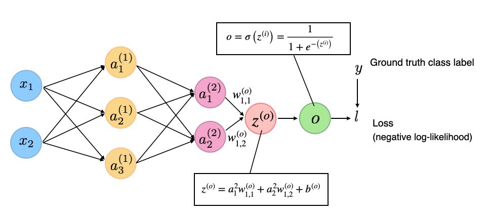
(Note that the superscript indices in the figure above are indexing the layers, not training examples.)

If you like this content and you are looking for similar, more polished Q & A’s, check out my new book Machine Learning Q and AI.