What is the difference between likelihood and probability?
Likelihood
Let’s start with defining the term likelihood. In everyday conversations the terms probability and likelihood mean the same thing. However, in a statistics or machine learning context, they are two different concepts.
Using the term probability, we calculate how probable (or likely) it is to draw a sample from a given distribution with certain parameters. For example, considering a continuous distribution like the normal distribution, we compute the probability as the area under the curve for a given range of values for the data \(x\). We do this by integrating the probability density function with fixed parameters: for the normal distribution, these parameters are the mean and standard deviation. The figure below illustrates this concept by calculating the probability of drawing a sample \(x\) with a value between 0 and 0.5 for a standard normal distribution (mean 0 and standard deviation 1), that is, \(Pr(0 < x < 0.5 \vert \mathbf{w}) =\int_{0}^{0.5} p(x \vert \mathbf{w}) dx\):
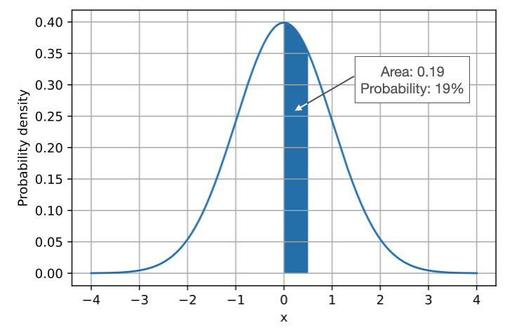
In general terms, we can define the probability density as \(p(\mathbf{x} \vert \mathbf{w})\), where \(\mathbf{x}\) is the data and \(\mathbf{w}\) are the parameters of a distribution or a model.
Side note
A normal distribution has the parameters \(\mu\) (mean) and \(\sigma\) (standard deviation); however I am using \(\mathbf{w}\) in \(\mathcal{L}(\mathbf{w} \vert \mathbf{x})\) instead of \(\mathcal{L}(\mu, \sigma \vert \mathbf{x})\) to keep it general. This will also make the notation is a bit more natural in a machine learning context later. For now, in the context of normal distributions you can think of it as follows: \(\mathbf{w} = (\mu, \sigma)\).
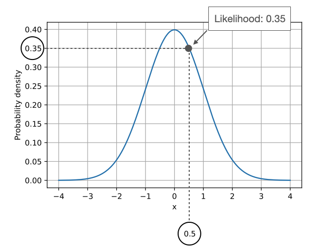
As illustrated by the previous figure, probability quantified how probable it is to sample data (\(\mathbf{x}\)) with certain values from a given distribution given the parameters (\(\mathbf{w}\)) of the distribution. On the other hand, the likelihood, \(\mathcal{L}(\mathbf{w} \vert \mathbf{x})\), computes how likely the parameters are given the observed data – in a practical context, we change the parameters of the distribution and see how it affects the likelihood. The figure below illustrates how we can obtain the likelihood of a fixed data point \(x=0.5\):
Notice the relationship between likelihood and probability density:
\(\mathcal{L}(\mathbf{w} \vert \mathbf{x}) = p(\mathbf{x} \vert \mathbf{w})\).
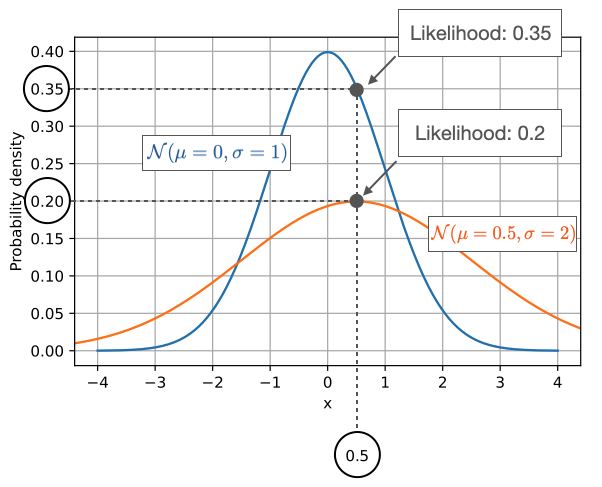
While the values are the same, the concepts are different. With probabilities (or probability densities), we assume given parameters and compute the probabilities in the context of sampling from a distribution. On the other hand, when we consider likelihoods, we regard the data as fixed and vary the parameters of the distribution. In many contexts, we are interested in finding the parameters that maximize the likelihood.
The following figure compares the likelihood of a fixed data point \(x=0.5\) for two different normal distributions: