How does a training loop in PyTorch look like?
A typical training loop in PyTorch
Let’s assume we are interested in training a deep neural network for supervised learning – it can be either classification or regression.
In PyTorch, a training loop typically looks like this:
model = MyNeuralNetwork(...)
optimizer = torch.optim.SGD(
  model.parameters(), lr=0.01, momentum=0.9
)

for epoch in range(num_epochs):
    for batch_idx, (features, targets) in enumerate(train_loader):

        forward_pass_outputs = model(features)
        loss = loss_fn(forward_pass_outputs, targets)
        optimizer.zero_grad()
        loss.backward()
        optimizer.step()
In the pseudo-code above, we have two for-loops to implement backpropagation with stochastic gradient descent-based optimization. The code nested under the inner for-loop (for batch_idx ...) defines a training step, which is also often just called “iteration.” In each iteration, we fetch a batch from the training dataset consisting of two tensors: the model inputs (features) and the targets. The model inputs are images in an image classification context, and the targets are the corresponding class labels. For example, the figure below illustrates the features and targets in a batch with an arbitrary batch size of 7:
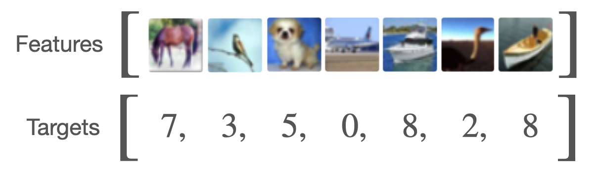
(Note that each image is itself a tensor 32x32x3 pixels, but this is perhaps too much detail.)
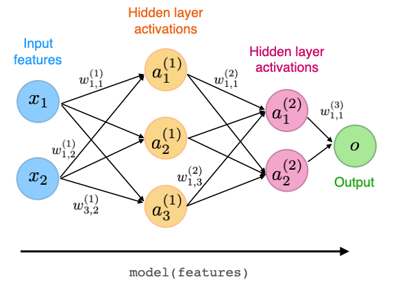
Next, model(features) executes the forward pass that computes the model outputs, and it constructs a computation graph behind the scenes. Here, model is an arbitrary supervised learning model. Note that we are purposefully vague about the return value forward_pass_outputs at this point. We will revisit this topic in a later section. The figure below illustrates the forward pass in the context of a simple, conceptual multilayer perceptron:
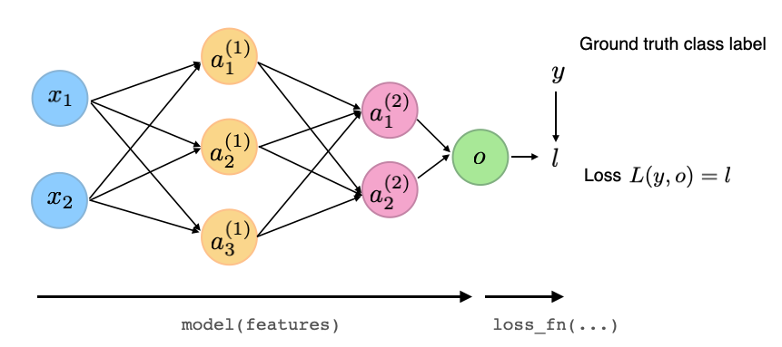
Via loss_fn, we then carry out a computation that measures the difference between the model outputs and the desired target values. This computation is added to the computation graph that exists behind the scenes. Similar to the return value of the model, we are purposefully vague about the definition of the loss function since we are establishing the bigger picture first. Technically, we can think of the loss computation as part of the forward pass during training, as illustrated below:
The following lines are where it gets interesting as they define the backpropagation procedure for training the neural network:
optimizer.zero_grad()
loss.backward()
optimizer.step()
The optimizer is typically an object for gradient descent-based optimization, for example, standard stochastic gradient descent, ADAM, etc.
When we perform backpropagation, PyTorch allows us to accumulate gradients – this is an advanced concept that is only relevant for certain types of optimization algorithms. However, since this option exists, we have to manually ensure that the gradients are reset to zero at in each backpropagation round. We do this via optimizer.zero_grad().
Calling loss.backward() will run reverse mode automatic differentiation on the computation graph defined in the forward pass (model(features) & loss_fn(...)). Calling loss.backward() will compute the gradient of the loss with respect to the weights, which are needed to update the weights using stochastic gradient descent, which happens in the next step when we call optimizer.step().
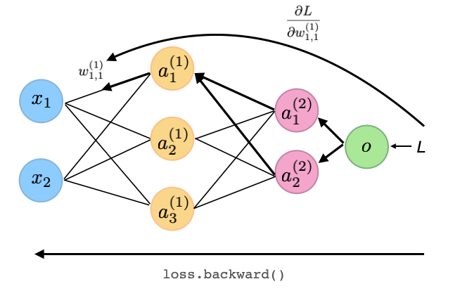
For illustration purposes, the following figure sketches the backpropagation step by highlighting all the connections that are involved in computing the gradient for one of the weights in the first hidden layer (this computation involves the multivariable chain rule):
Finally, the outer for-loop (for epoch in range(num_epochs):) repeats the batch iteration and training steps for multiple passes over the training set (epoch is really just a fancy term for defining a pass over a training set, visiting each training example exactly once.)
Training loop summary
To recap and summarize, a typical training loop in PyTorch iterates over the batches for a given number of epochs. In each batch iteration, we first compute the forward pass to obtain the neural network outputs:
forward_pass_outputs = model(features)
loss = loss_fn(forward_pass_outputs, targets)
Then, we reset the gradient from the previous iteration and perform backpropagation to obtain the gradient of the loss with respect to the model weights:
optimizer.zero_grad()
loss.backward()
Finally, we update the weights based on the loss gradients using stochastic gradient descent:
optimizer.step()
Bonus: A training loop in PyTorch Lightning
If we are using PyTorch Lightning, we don’t have to worry about defining the training loop as it takes care of it for us.
What is Pytorch Lightning?
PyTorch Lightning is a library that helps you organize your PyTorch code, reduce boilerplate, and makes several best and advanced practices, such as logging, checkpointing, and multi-GPU training easier.
The following minimal example shows the previous PyTorch example in a PyTorch Lightning context:
import pytorch_lightning as pl


# LightningModule that receives a PyTorch model as input
class LightningModel(pl.LightningModule):
    def __init__(self, model, ...):
        super().__init__()
        ...

    def training_step(self, batch, batch_idx):
        features, targets = batch
        forward_pass_outputs = model(features)
        loss = loss_fn(forward_pass_outputs, targets)
				...
        return loss  # this is passed to the optimzer for training

    ...

    def configure_optimizers(self):
        optimizer = torch.optim.SGD(self.parameters(), lr=self.learning_rate)
        return optimizer

...
trainer = pl.Trainer(
    max_epochs=NUM_EPOCHS,
    ...
)

lightning_model = LightningModel(pytorch_model, ...)
trainer.fit(model=lightning_model, ...)
(If you are interested, I have a full, self-contained example here.)
In PyTorch Lightning, we define the code for a step in the training loop inside the training_step method. Notice that this is the same pseudo-code that we used in the previous section to define the forward pass. Now, we don’t have to worry about the backward pass, which the Trainer handles automatically for us upon calling trainer.fit(...).