
Short Convolution (ShortConv)
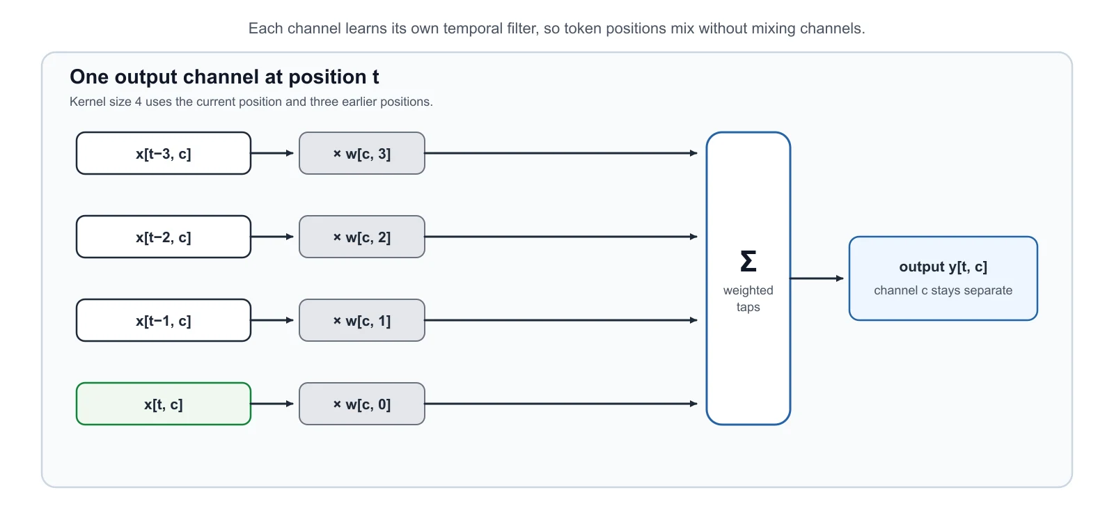
I find ShortConv easiest to understand by ignoring the full model for a moment. Take one hidden channel and look at four adjacent token positions. ShortConv multiplies those four values by four learned weights and adds them. That’s essentially it.
Kimi Linear and Inkling both use a kernel size of 4. Since the convolution is causal, the four positions are the current token and the three preceding tokens.
The convolution is also depthwise. Each hidden channel has its own weights; the surrounding linear projections handle the cross-channel mixing. The two models use this same operation in very different places.
Local receptive field
The current token plus the three preceding positions when the kernel size is 4
Decode state
A fixed-size rolling state whose size does not grow with the context length
Example architectures
How a causal depthwise ShortConv works
For one channel c and a kernel size k, the convolution at position t is
y[t, c] = Σᵢ w[c, i] · x[t - i, c] for i = 0, ..., k - 1
The word causal means that future tokens are off limits. At the beginning of the sequence, missing earlier values are zeros. For k = 4, the four inputs are x[t], x[t-1], x[t-2], and x[t-3].
The word depthwise means that channel c does not read another channel during this step. A dense projection can still mix all channels before or after the convolution.
A minimal PyTorch version
The code below implements this operation. The activation and residual switches cover the two model-specific variants discussed later.
import torch
import torch.nn as nn
import torch.nn.functional as F


class ShortConv(nn.Module):
    def __init__(self, d_model, kernel_size=4, activation=None, residual=False):
        super().__init__()
        self.kernel_size = kernel_size
        self.activation = activation
        self.residual = residual
        self.conv = nn.Conv1d(
            in_channels=d_model,
            out_channels=d_model,
            kernel_size=kernel_size,
            groups=d_model,
            bias=False,
            padding=kernel_size - 1,
        )

    def forward(self, x):
        # x has shape (batch, tokens, channels)
        y = self.conv(x.transpose(1, 2))
        y = y[:, :, : x.shape[1]].transpose(1, 2)

        if self.activation == "silu":
            y = F.silu(y)
        if self.residual:
            y = y + x
        return y
Conv1d pads both sides of the sequence. The truncation removes outputs that depend on right-side padding and keeps the result causal.
Why the operation is cheap
Why bother adding this small layer? One reason is cost. For T tokens, hidden width d, and kernel size k, the work is roughly O(Tdk). With k = 4, it grows linearly with sequence length.
At inference, the model keeps a small rolling state with the recent activations. The state is O(dk), so it does not grow with the context. ShortConv handles local mixing; attention remains responsible for broader retrieval.
How ShortConv complements KDA
The convolution is only one part of Kimi Delta Attention (KDA). KDA is a refinement of Gated DeltaNet, so it helps to briefly look at what this recurrent attention family does and why a separate local mixing step is useful.
Now, what is Gated DeltaNet? Gated DeltaNet (short for Gated Delta Network) is Qwen3-Next’s linear-attention layer, which is intended as an alternative to standard softmax attention. It was adopted from the Gated Delta Networks: Improving Mamba2 with Delta Rule paper.
Gated DeltaNet was originally proposed as an improved version of Mamba2, where it combines the gated decay mechanism of Mamba2 with a delta rule. The delta rule part refers to computing the difference (delta) between new and predicted values to update a hidden state that is used as a memory state.
KDA changes parts of this mechanism, including the decay gate, but keeps the recurrent state-update idea. ShortConv sits immediately before that update in Kimi Linear.
In gated attention, the model computes normal attention between all tokens (every token attends or looks at every other token). Then, after getting the attention output, a gate (a sigmoid) decides how much of that output to keep. The takeaway is that it’s still the regular scaled-dot product attention that scales quadratically with the context length.
As a refresher, scaled-dot product attention is computed as softmax(QKᵀ)V, where Q and K are n-by-d matrices, where n is the number of input tokens, and d is the embedding dimension. So QKᵀ results in an attention n-by-n matrix that is multiplied by an n-by-d dimensional value matrix V.
In Gated DeltaNet, there’s no n-by-n attention matrix. Instead, the model processes tokens one by one. It keeps a running memory (a state) that gets updated as each new token comes in.
The gates control how that memory changes:
- α (alpha) regulates how much of the old memory to forget (decay)
- β (beta) regulates how much the current token at time step t updates the memory
The final output gate is similar to gated attention; it controls how much of the output is kept.
In a sense, this state update in Gated DeltaNet is similar to how recurrent neural networks (RNNs) work. The advantage is that it scales linearly, instead of quadratically, with context length.
The downside of the recurrent state update is that, compared to regular or gated attention, it sacrifices the global context modeling ability that comes from full pairwise attention. Gated DeltaNet can still capture context, but it has to go through the memory bottleneck. That memory is a fixed size and thus more efficient, but it compresses past context into a single hidden state similar to RNNs.
This is why Kimi Linear uses a hybrid setup instead of replacing every attention layer with KDA. Its 20 KDA layers handle the efficient recurrent updates, and the 7 MLA layers retain full-attention-style retrieval. Within a KDA layer, ShortConv adds a direct four-token mixing path before the recurrent update.
There is a similar distinction at inference. ShortConv keeps only the recent k - 1 activations per channel. The recurrent attention mechanism keeps its fixed-size memory state. Neither state grows with the number of tokens, although they serve different purposes: ShortConv preserves exact local activations, while the recurrent state compresses information carried across longer ranges.
Next to the linear compute complexity, another big advantage of the recurrent mechanism is the memory savings, as these layers don’t grow the KV cache. Instead, as mentioned earlier, they keep a fixed-size recurrent state, so memory stays constant with context length.
For a regular multi-head attention (MHA) layer, we can compute the KV cache size as follows:
KV_cache_MHA ≈ batch_size × n_tokens × n_heads × d_head × 2 × bytes
The factor of 2 is there because we store both keys and values. For a simplified DeltaNet layer, the state size is
state_DeltaNet = batch_size × n_heads × d_head × d_head × bytes
The second expression doesn’t have a context-length (n_tokens) dependency. Also, there is only one memory state instead of separate keys and values. However, it has a quadratic d_head × d_head term. That’s usually nothing to worry about because the head dimension is relatively small. For instance, it’s 128 in Qwen3-Next.
The full recurrent mechanism, including the convolutional mixing, is more complex. Still, these formulas show the main trend: the recurrent state carries compressed long-range information, while ShortConv contributes a much smaller rolling buffer for exact local mixing.
Kimi Linear shares several structural similarities with Qwen3-Next. Both models rely on a hybrid attention strategy. Concretely, they combine lightweight linear attention with heavier full attention layers. Both use an approximately 3:1 ratio, meaning that roughly three recurrent linear-attention blocks are paired with one full-attention block.
Gated DeltaNet is a linear-attention variant with inspiration from recurrent neural networks, including a gating mechanism from the Gated Delta Networks paper. In a sense, Gated DeltaNet is a DeltaNet with Mamba-style gating, and DeltaNet is a linear-attention mechanism.
Kimi Linear modifies this mechanism with KDA. Whereas Qwen3-Next applies a scalar gate (one value per attention head) to control the memory decay rate, Kimi Linear replaces it with channel-wise gating for each feature dimension. The Kimi Linear paper argues that this gives more control over the memory and, in turn, improves long-context reasoning.
For the full-attention layers, Kimi Linear uses multi-head latent attention (MLA), the same general mechanism used by DeepSeek V3 and R1, but with an additional gate. MLA compresses the key/value space to reduce the KV cache size. These MLA layers provide the global attention path in the hybrid. They don’t contain the three Q/K/V ShortConv modules shown in the KDA path.
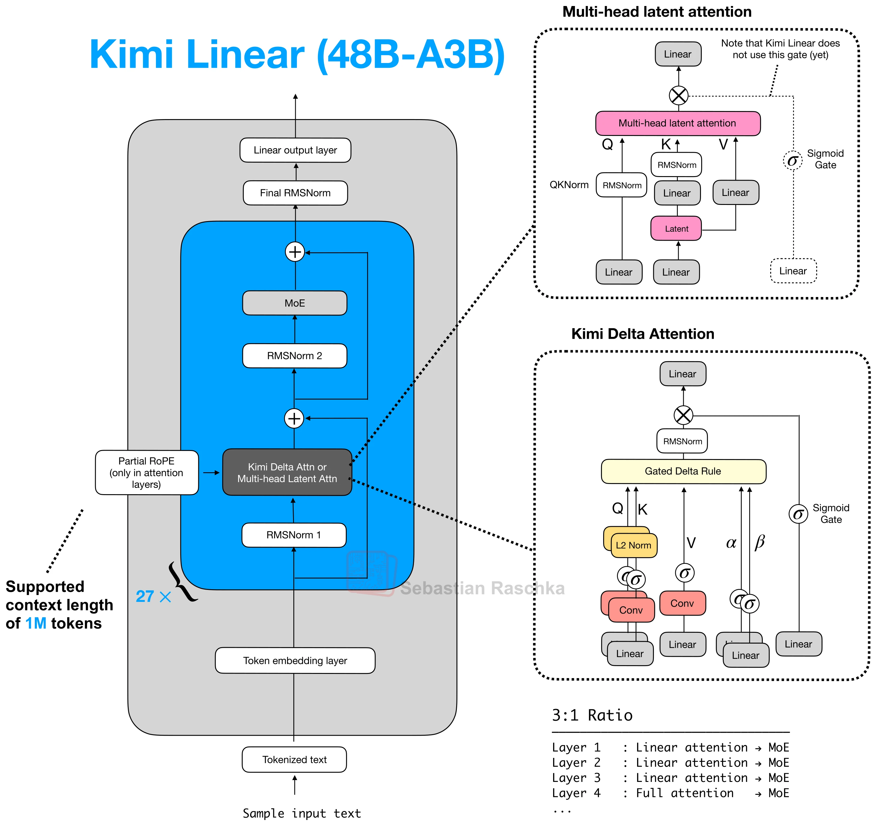
Kimi Linear filters Q, K, and V in KDA layers
Kimi Linear’s use of ShortConv is quite specific. Of its 27 decoder layers, 20 use Kimi Delta Attention (KDA) and 7 use MLA.
Each KDA layer has three ShortConv modules, one each after the Q, K, and V projections. The three convolutions use a kernel size of 4 and a SiLU activation. Their outputs go into the recurrent KDA update. The 7 MLA layers do not use them.
In short, the four-token mixing happens before the recurrent state update.
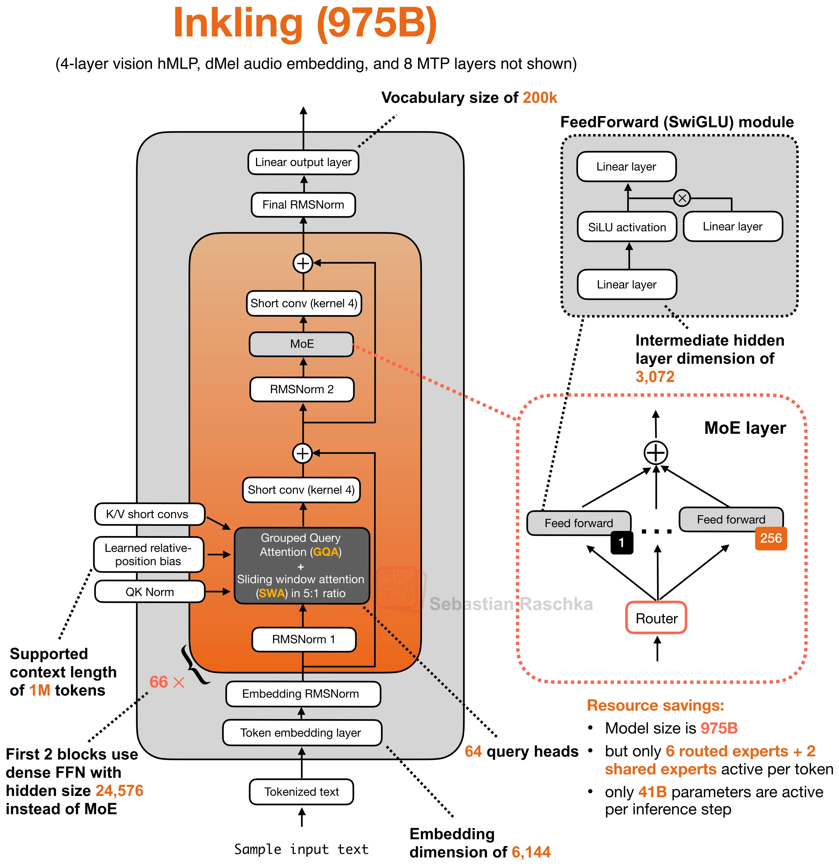
Inkling uses four ShortConv modules in every layer
Inkling goes further. It uses four ShortConv modules in each of its 66 decoder layers:
-
k_sconvafter the key projection -
v_sconvafter the value projection -
attn_sconvafter the attention output and before the main residual addition -
mlp_sconvafter the MLP or MoE output and before the main residual addition
The kernel size is again 4. Inkling adds each module input back to the convolution output, giving it a small residual path. The Hugging Face implementation also keeps these convolutions in FP32.
The K and V modules mix neighboring tokens inside attention. The other two do the same after attention and after the feed-forward computation.
Same kernel, different placement
For Kimi Linear, ShortConv prepares Q, K, and V inside KDA. For Inkling, it affects K, V, and both residual branch outputs. The kernel is the same; the placement is the main difference.
Why Kimi Linear still retains full attention
In those older systems, an encoder RNN would read the source sentence token by token and compress it into a sequence of hidden states, or in the simplest version into one final state. Then the decoder RNN had to generate the target sentence from that limited summary. This worked for short and simple cases, but it created an obvious bottleneck once the relevant information for the next output word lived somewhere else in the input sentence.
In short, the limitation is that the hidden state can’t store infinitely much information or context, and sometimes it would be useful to just refer back to the full input sequence.
The translation example below shows one of the limitations of this idea. For instance, a sentence can preserve many locally reasonable word choices and still fail as a translation when the model treats the problem too much like a word-by-word mapping. (The top panel shows an exaggerated example where we translate the sentence word by word; obviously, the grammar in the resulting sentence is wrong.) In reality, the correct next word depends on sentence-level structure and on which earlier source words matter at that step. Of course, this could still be translated fine with an RNN, but it would struggle with longer sequences or knowledge retrieval tasks because the hidden state can only store so much information as mentioned earlier.
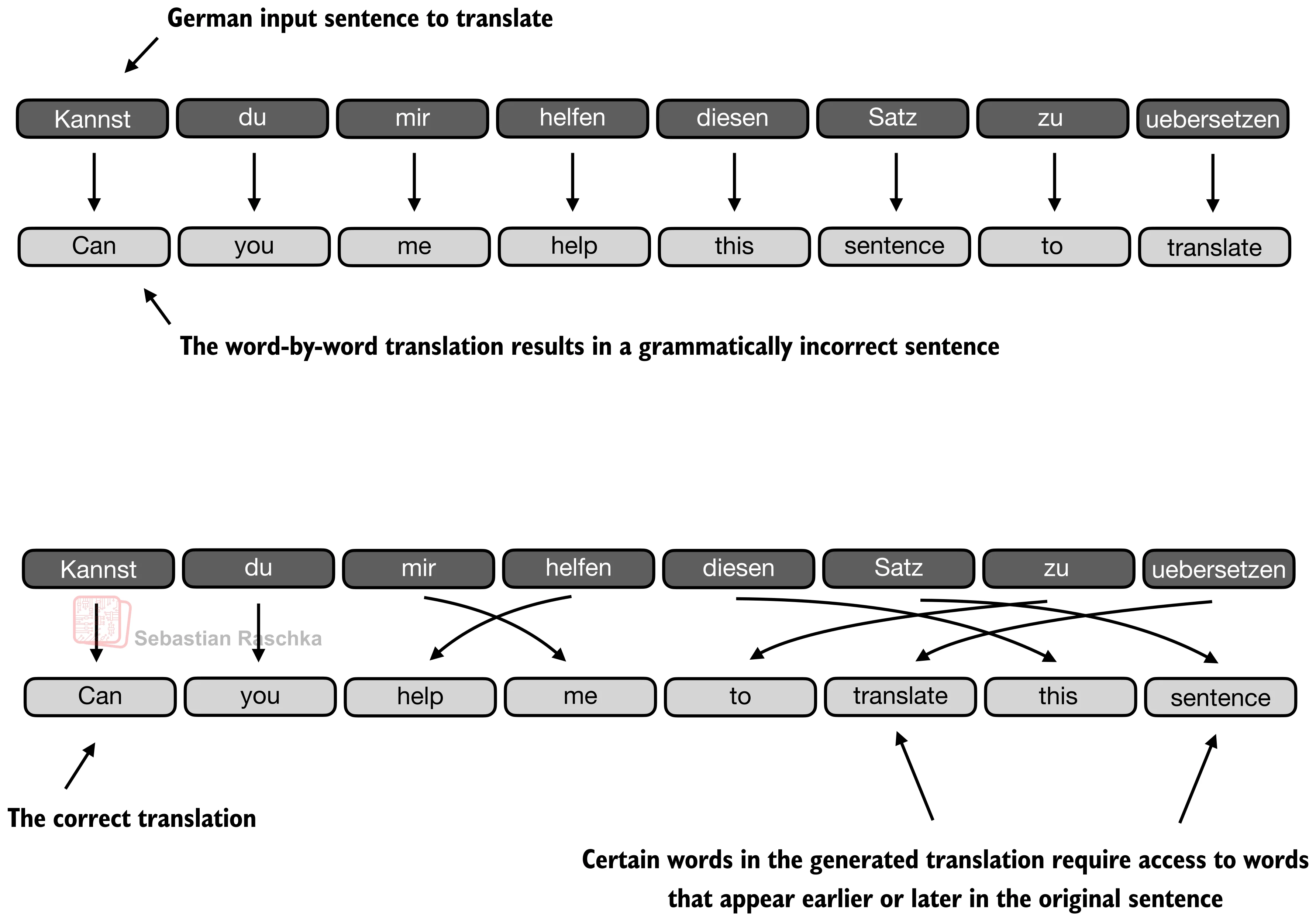
So, to overcome the limitation of standard RNNs, that everything gets stored in a hidden state, and that the model can’t access the original inputs when needed, researchers added an attention mechanism via Neural Machine Translation by Jointly Learning to Align and Translate. The point was to remove that fixed-summary bottleneck of the hidden state and instead of forcing the decoder to rely on one compressed summary of the whole input, attention lets it build a step-specific context vector at each output step by revisiting the more relevant encoder states.
In language, this matters because the word we want next often depends on content that appeared much earlier or later in the source sentence, not just on the immediately previous token.
Kimi Linear keeps seven MLA layers for this full-attention path. Its other twenty layers use the more efficient recurrent KDA path, with ShortConv providing the local four-token mixing described above.
Sources