
Appendix to Understanding Positional Embeddings in Modern LLMs
This page contains supplementary material for the Understanding Positional Embeddings in Modern LLMs article. Concretely, it covers some additional explainers including the token embedding lookup and attention calculations. Also, it covers some more experimental result discussions that compare the different positional methods. And it also explains how long-context support is often improved via rescaling RoPE with YaRN.
Appendix A. Token embedding lookups
This appendix further illustrates the difference between a token ID and a position index from Section 1.1. For this example, we use the same sentence, “The red fox jumps over the gray fox”, and for simplicity, we continue to assume that 1 token = 1 word.
Figure A.1 below shows an illustration with a small toy vocabulary with seven entries (as mentioned in the main article, a real vocabulary has between 50k and 200k entries, but this would be hard to visualize). Each token ID, independent of where it is located in the input text, selects a row from the learned embedding table, which starts out as a random weight matrix and is updated during training.
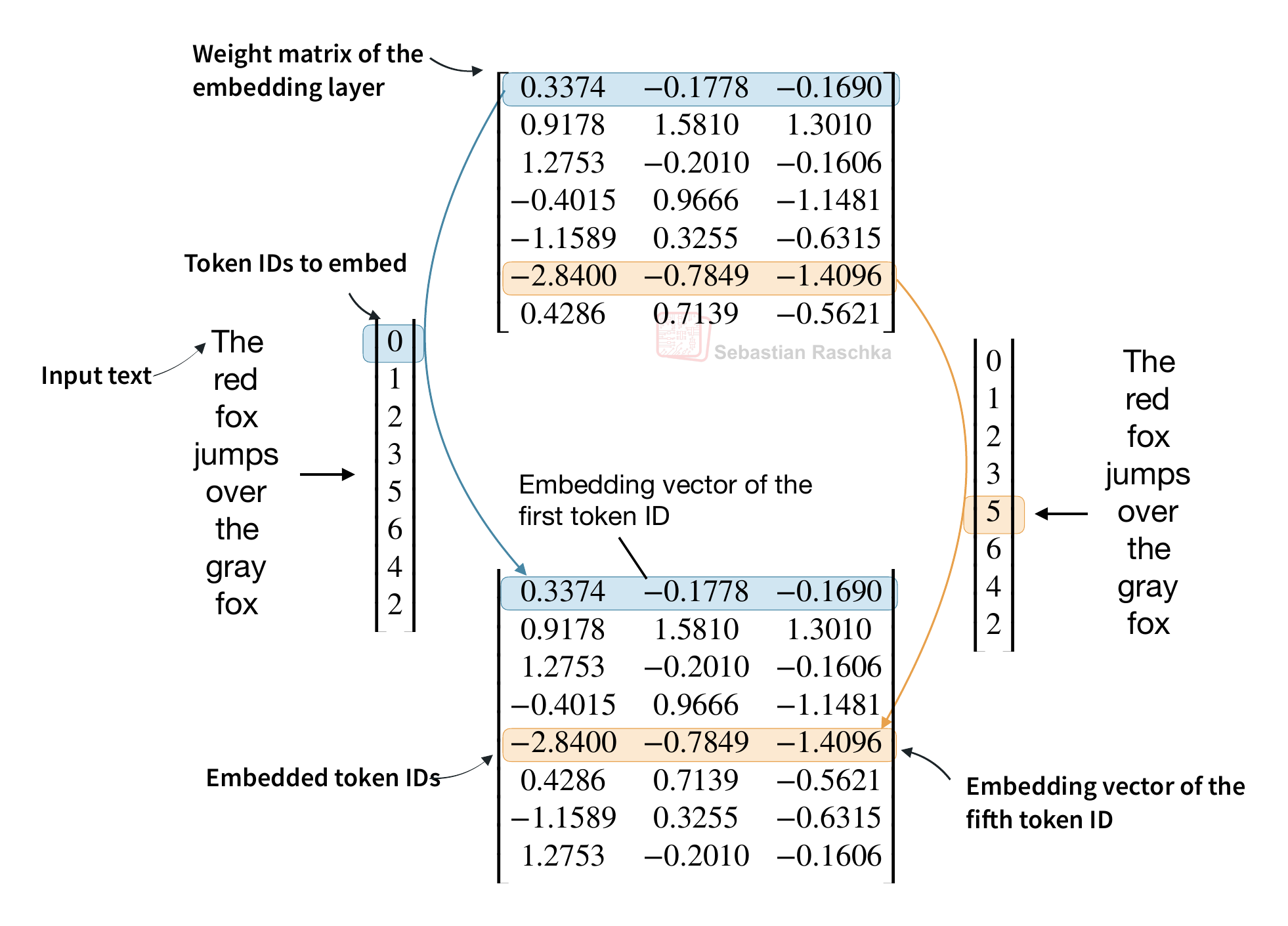
For instance, the sentence “The red fox jumps over the gray fox” results in the following sequence of token IDs [0, 1, 2, 3, 5, 6, 4, 2]. Then, as shown in the figure above, we select the corresponding rows, using zero-based indexing, from the embedding table. For example, ID 2 for “fox” selects the third row, [1.2753, -0.2010, -0.1606]. This selection is based on the fact that the token ID for “fox” is 2 based on the vocabulary not because it is in index position 2.
To make this more clear, consider the second entry for “fox” in the last position of the sentence. Both occurrences of “fox” have vocabulary ID 2, even though they appear at positions 2 and 7, as shown in Figure A.2.
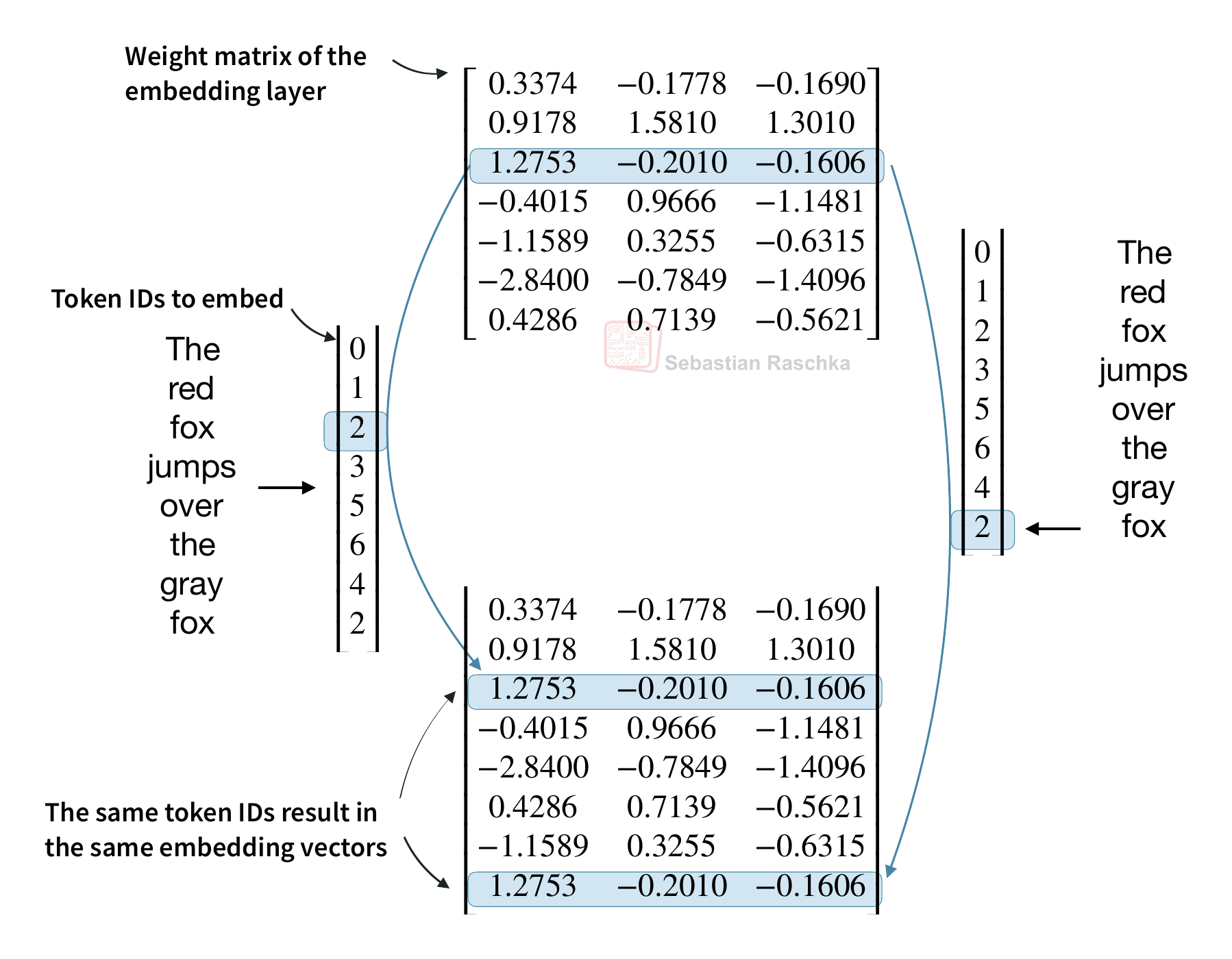
So, as shown in the figure above, both occurrences of “fox” receive the same embedding vector since they both have the same token ID. In other words, the embedding lookup depends only on the token ID, so it doesn’t tell us where that token occurs in the input. Now, swapping the two words “red” and “gray” in our sentence rearranges the order in which we obtain the resulting embedding vector from the embedding table, but it doesn’t change the embedding vectors for “red” and “gray,” respectively.
As mentioned, the embedding tables (implemented as an embedding layer in PyTorch) are updated during training,s o the these vector entries are learned numerical features.
Appendix B. Attention, masks, and position information
This appendix section works through the attention example from Section 1.1. Here, keep the token embeddings fixed and compare the query at “jumps” in two sentences from earlier: “The red fox jumps over the gray fox” and “The gray fox jumps over the red fox.”
B.1 Unrestricted attention
Let’s start with an unrestricted vanilla attention example, meaning no causal mask. Here, every token can attend to every token (including itself) as shown in the figure below.
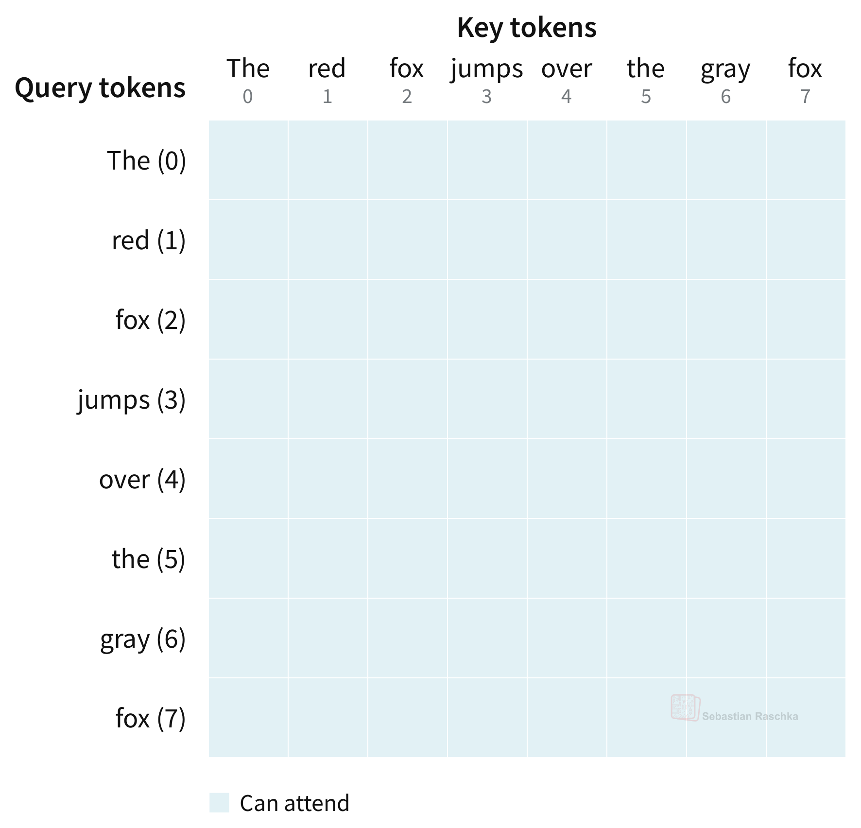
Now we do a little experiment where we swap red and gray and look at the attention output for jumps. (Following the figures below, I also included a code snippet to reproduce this.)
In the attention mechanism without causal mask, and with no positional encoding, the first-layer query for jumps sees the same keys and values in a different order. Note that the weights move with their value vectors, so the weighted sum in Figure B.2 stays exactly the same.
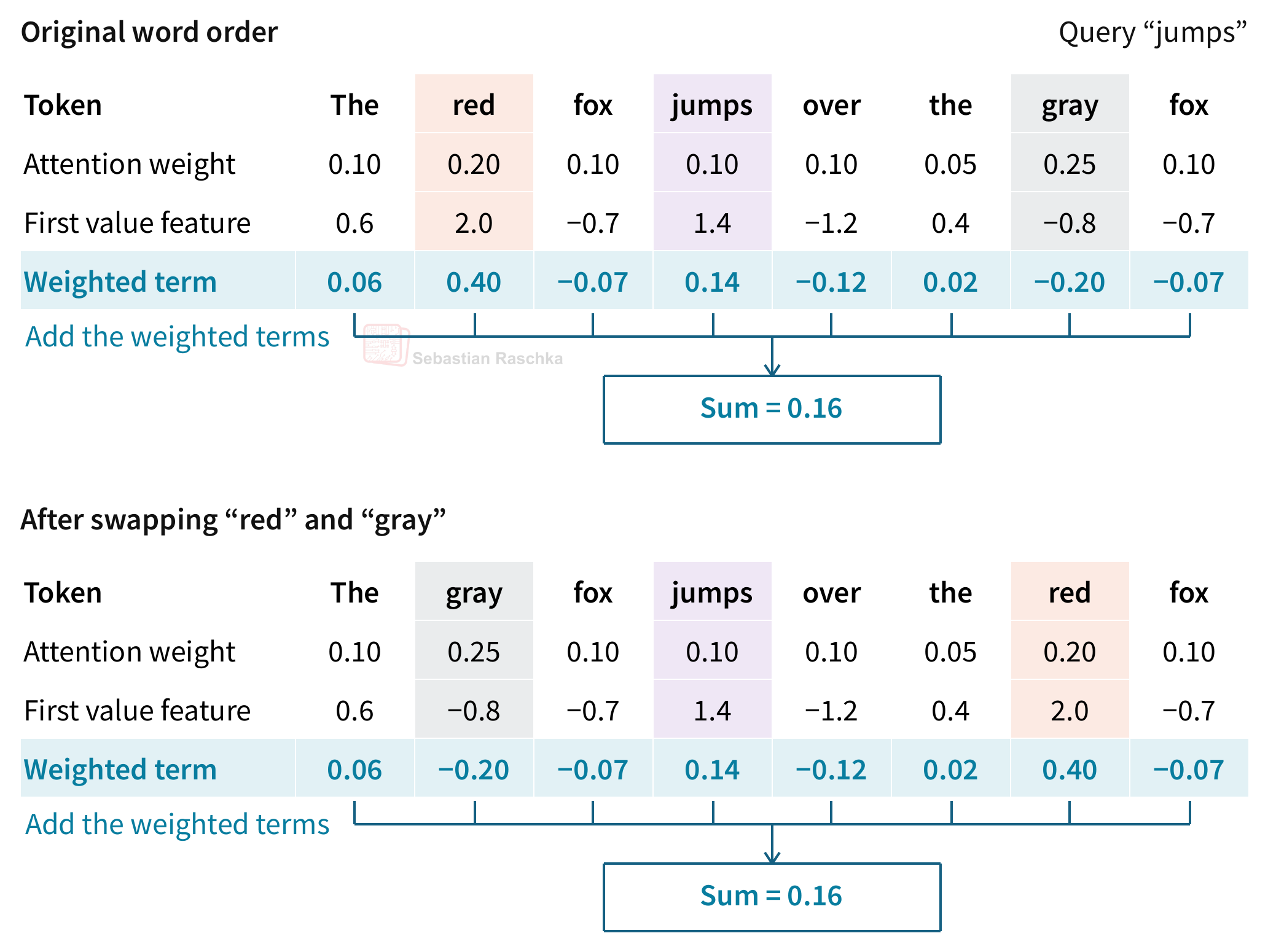
If you want to reproduce these numbers, here’s the PyTorch code for the example in the figure above with some hard-coded numbers for the raw attention scores (scores) and value vectors (value_features) chose toy scores for the query at jumps by taking the log of small integers.
import torch

tokens = "The red fox jumps over the gray fox".split()

# Toy scaled query-key scores and one value feature per key.
scores = torch.tensor([2.0, 4.0, 2.0, 2.0, 2.0, 1.0, 5.0, 2.0]).log()
value_features = torch.tensor([0.6, 2.0, -0.7, 1.4, -1.2, 0.4, -0.8, -0.7])

original_order = torch.arange(len(tokens))
swapped_order = torch.tensor([0, 6, 2, 3, 4, 5, 1, 7])  # Swap red and gray.

# The comments under each print show the original order, then the swapped order.
for order in (original_order, swapped_order):
    weights = scores[order].softmax(dim=0)
    ordered_features = value_features[order]
    weighted_terms = weights * ordered_features

    print("Tokens:", " ".join(tokens[i] for i in order.tolist()))
    # Tokens: The red fox jumps over the gray fox
    # Tokens: The gray fox jumps over the red fox

    print("Weights:", [round(w, 2) for w in weights.tolist()])
    # Weights: [0.1, 0.2, 0.1, 0.1, 0.1, 0.05, 0.25, 0.1]
    # Weights: [0.1, 0.25, 0.1, 0.1, 0.1, 0.05, 0.2, 0.1]

    print("First value feature:", [round(v, 1) for v in ordered_features.tolist()])
    # First value feature: [0.6, 2.0, -0.7, 1.4, -1.2, 0.4, -0.8, -0.7]
    # First value feature: [0.6, -0.8, -0.7, 1.4, -1.2, 0.4, 2.0, -0.7]

    print("Weighted terms:", [round(t, 2) for t in weighted_terms.tolist()])
    # Weighted terms: [0.06, 0.4, -0.07, 0.14, -0.12, 0.02, -0.2, -0.07]
    # Weighted terms: [0.06, -0.2, -0.07, 0.14, -0.12, 0.02, 0.4, -0.07]

    print(f"Weighted sum: {weighted_terms.sum().item():.2f}")
    # Weighted sum: 0.16 (both orders)
B.2 Adding a causal mask
Now let’s consider an attention mechanism with a causal mask. For example, in the causal case in the figure below, the query for jumps at position 3 can only attend to The, red, fox, and itself instead of any of the tokens that come after.
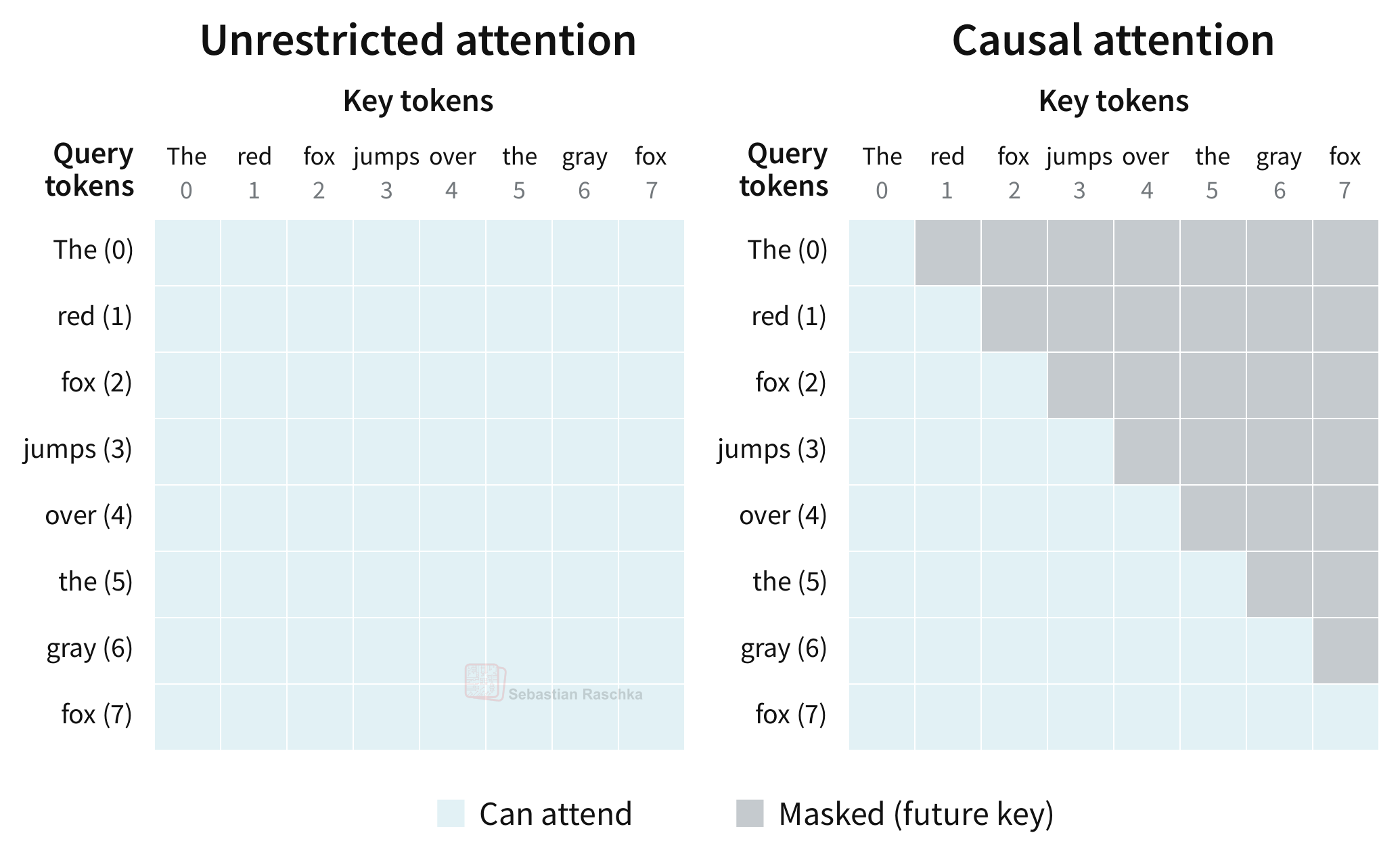
Let’s return to our two sentences, “The red fox jumps over the gray fox” and “The gray fox jumps over the red fox.” With the causal mask (as depicted in the right subpanel o f the previous figure), jumps can attend to red in the first sentence and gray in the second.
Now, to make things concrete, Figure B.4 below uses the same unmasked scores and value features as Figure B.2, but softmax now runs over the non-masked tokens only.
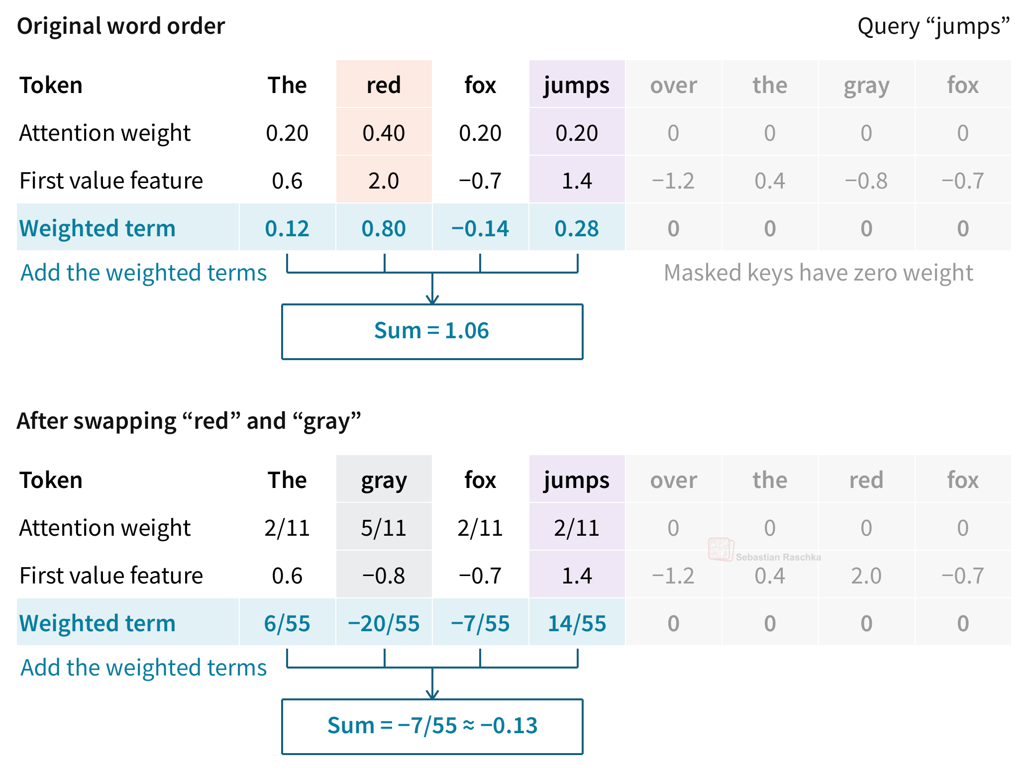
The illustrated output feature changes from 1.06 to approximately -0.13. So, we can see that the mask supplies an implicit source of order information, even though there is no explicit positional encoding.
B.3 What explicit position information adds
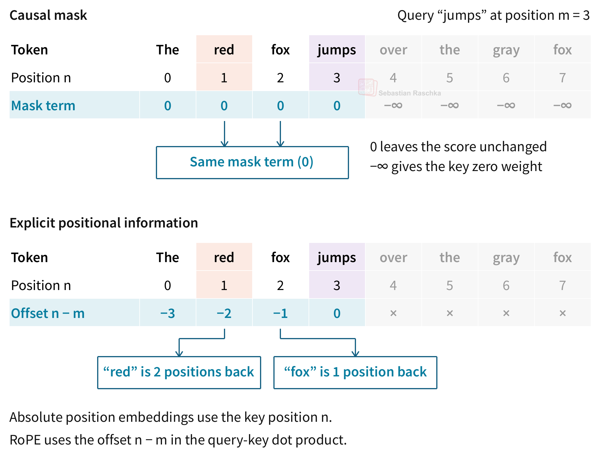
The previous causal mask assigns a placeholder-score of 0 to every non-masked pair and negative infinity to every masked pair (see my Build A Large Language Model (From Scratch) book for details on the underlying math and why). For the query “jumps” at position 3, both “red” at position 1 and “fox” at position 2 are allowed. They receive the same “mask adjustment”, despite being at different distances.
Appendix C. What comparative experiments show
The main article focused on how the various mechanisms work, but how well do they do and how do they compare in practice / empirically? Below are some additional comparisons. Unfortunately, the ablation studies and comparisons are scarce, old, oder on a small scale, but it’s still better than nothing.
C.1 Learned versus sinusoidal position vectors
The original GPT models used learned position embeddings, but the papers didn’t state any reasons why choosing them over the sinusoids used in the original transformer architecture. However, there are some other studies that compare the two methods (including the original transformer paper):
| Study and evaluation setting | Metric | Fixed sinusoidal | Learned absolute |
|---|---|---|---|
| Vaswani et al. (2017), Table 3, base transformer, English-to-German dev set | BLEU, higher is better | 25.8 | 25.7 |
| Same translation experiment | Wordpiece perplexity, lower is better | 4.92 | 4.92 |
| Haviv et al. (2022), Table 1, WikiText-103, 512-token sequences | Validation perplexity, lower is better | 20.16 | 20.42 |
| Same study, 1.3B-parameter GPT-3-style model, Pile subset, 1,024-token sequences | Validation perplexity, lower is better | 12.93 | 13.05 |
These results don’t show a general quality advantage for learned embeddings. Actually, the later language-model experiments slightly favor sinusoids. So one might think it all came down to simplicity and convenience.
There is, however, evidence that learned embeddings can capture useful positional relationships. For instance, Wang and Chen (2020) trained a simple classifier that takes position embeddings as input and predicts which of two positions came first. Figure C.1 below shows the setup.
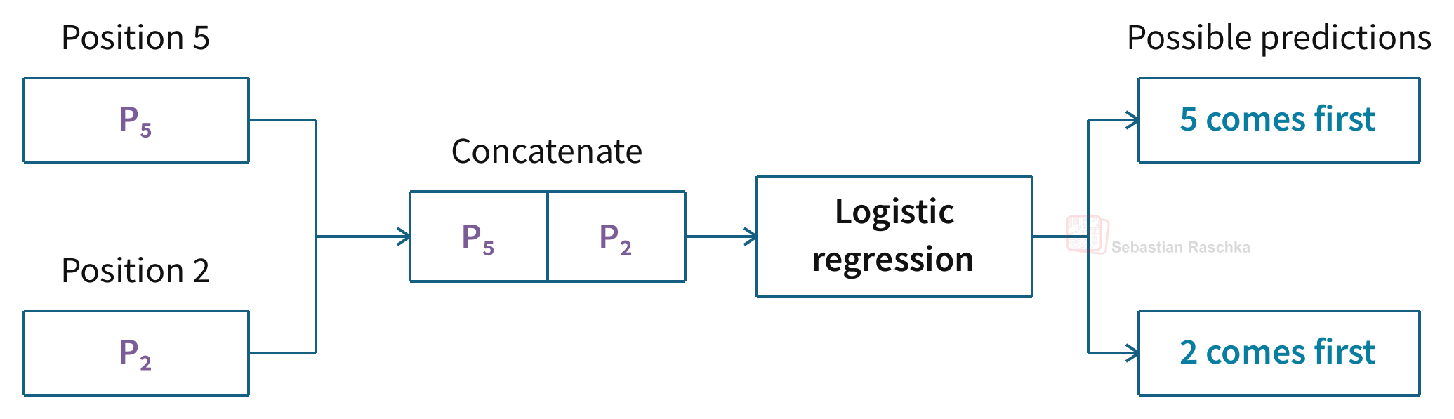
The classifier had a 1.56% error rate when using the pretrained GPT-2 position embedding vectors, and it had a noticeably worse 5.08% error rate for sinusoidal vectors. However, keep in that this doesn’t establish that learned embeddings improve language-model quality.
Anyways, my explanation why GPT used the learned position vectors is that it was a simple and straightforward thing to do, plus, with the smaller contexts lengths back then (512 tokens for GPT-1, 1024 tokens for GPT-2), this was also a reasonable thing to do at the time.,
C.2 RoPE and ALiBi
ALiBi (short for Attention with Linear Biases) is an alternative positional embedding method that enjoyed some popularityh a few years ago, roughly around the same time RoPE was becoming popular.
It works like this. Before softmax, it subtracts a penalty from the scaled query-key dot product. Just considering each head individually, that penalty grows by a fixed amount for every position difference between the key and the query. So a key two positions back gets twice the penalty of a key one position back.
If this looks familiar, Inkling adds its learned position bias at the same point in the attention calculation as mentione in Section 6.3 of the main article.
How ALiBi changes attention scores
To illustrate ALiBi with a numerical example, let’s use our fox sentence. For the example in Figure C.2 below, we only need the first five tokens, The red fox jumps over. The query comes from jumps at position 3.
Now, if we subtract 0.5 for every position counting backwards from jumps, we subtract 1.0 for red (two positions back) and 0.5 for fox (one position back). The bias for jumps itself is zero. And since the over token is positioned after the query, the causal mask gives it an attention weight of zero.
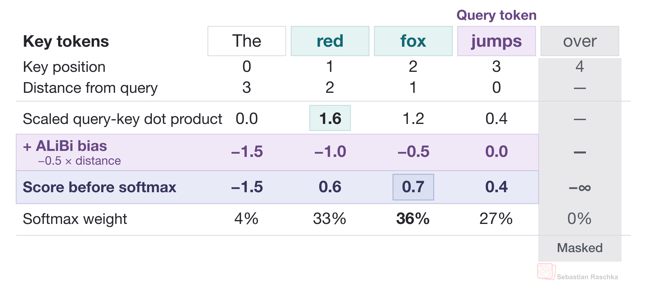
As we can see in the figure above, red starts out with a higher scaled dot product than fox (1.6 versus 1.2). After we add the biases, the scores are 0.6 and 0.7, respectively. So, after softmax, fox gets about 36% of the attention weight, and red gets about 33%. But of course, this doesn’t mean that the attention weight is entirely determined by position; if a key further away has a large enough dot product to begin with, it can still get the highest weight.
For those who prefer this concept spelled out in math symbols, let’s write the query position as \(m\) and the key position as \(n\). For a key the causal mask allows (\(n \leq m\)), the score in head \(h\) is
\[\text{score}_{m,n}^{(h)} = \frac{q_m^\top k_n}{\sqrt{d_k}} - a_h(m-n).\]The first qk term is the usual dot product divided by the square root of the key dimension \(d_k\). The second term subtracts the head’s slope \(a_h\) times the distance \(m-n\). In the example above, \(a_h\) was 0.5.
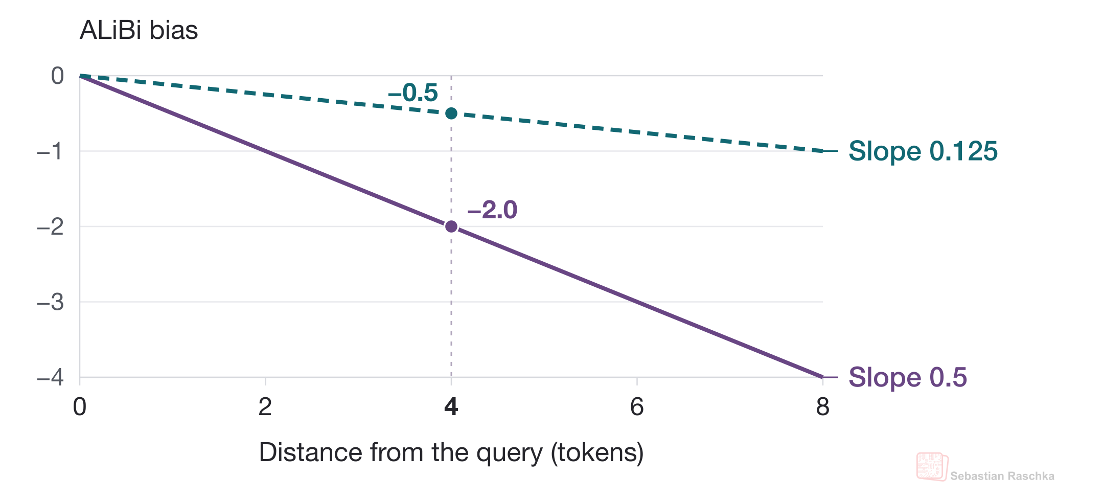
So, do all heads use the same slope for these biases? The original paper gives each head its own slope (at initialization, and keeping it fixed throughout training and afterwards). For eight heads, the slopes are \(1/2, 1/4, \ldots, 1/256\). Figure C.3 shows what this means for two of those heads. If the key is four positions back, the head with slope 0.5 subtracts 2 from its score, and the head with slope 0.125 subtracts only 0.5. So one head favors recent keys more strongly than the other.
Comparing positional methods
The RoFormer paper (see table 1) reported a small improvement on WMT 2014 English-to-German translation, from 27.3 BLEU for the sinusoidal baseline to 27.5 with RoPE, where a higher BLEU is better.
For causal language models, the GPT-NeoX-20B paper explicitly cited the team’s positive prior experience training with RoPE as its reason for replacing learned position embeddings, but there is no concrete empirical data.
So how does RoPE now compare with ALiBi? The original ALiBi paper included both methods in an ablation with 1.3B-parameter models trained on 112B tokens from OSCAR. Average zero-shot accuracy was 43.70% with ALiBi, 41.46% with RoPE, and 41.71% with learned position embeddings. So, ALiBi does come out ahead in this comparison.
Comparing RoPE and ALiBi on longer sequences
ALiBi’s bias calculation still works when the token gap is larger than any gap the model saw in training. We can just plug a larger number into the same formula. So how did ALiBi compare with RoPE on longer inputs?
In another experiment, the authors trained the models on 512-token sequences from WikiText-103. With RoPE, the validation perplexity went from 20.07 at 512 tokens to 19.79 at 712 tokens (a small improvement, since lower is better). By 2,512 tokens, it had risen to 31.58. With ALiBi, it went from 19.73 at 512 tokens to 18.41 at 2,512 tokens. So, again, ALiBi comes out ahead.
PS: We’ll come back to the question of longer inputs in Appendix D, where we’ll look at how YaRN adapts RoPE.
Why ALiBi is less common today
ALiBi made it into several well-known LLMs, including BLOOM in 2022 and MPT in 2023. In the November 9, 2026 snapshot I used for the main article, though, none of the 119 gallery entries released from 2024 onward uses ALiBi in its text decoder’s softmax attention, and it seems it’s fallen out of fashion. But why?
The results above also depend on what we measure. In the Falcon team’s ablations, RoPE had an edge at 1B parameters, and the performance gap shrank when considering the larger 3B model. There was also a tradeoff when a model needs to access tokens at the very back of a context window. For instance, as mentioned earlier, ALiBi’s penalty keeps increasing with distance, so in some attention heads, the attention weight for a distant token can round to zero, which is problematic. A 2026 preprint confirmed that this can indeed hurt retrieval (think of “needle-in-the-haystack” tasks) even when standard benchmarks change very little.
Another reason we teams now stick with RoPE is that LLMs have growing context sizes. For instance, Llama 3 increased the RoPE base to support longer sequences, and YaRN (covered further below in Appendix D) showed how to extend the context of a model that was already trained with RoPE, so I guess it made it easier to just keep the same positional method as context windows grew.
C.3 Evidence for NoPE
Kazemnejad et al. (2023) tested whether NoPE learns useful positional behavior in practice. In this research article, the authors trained smallish 107M-parameter LLMs from scratch on ten reasoning and algorithmic tasks. Then, they evaluated generalization to longer inputs. The aggregate results are shown in the figure below.
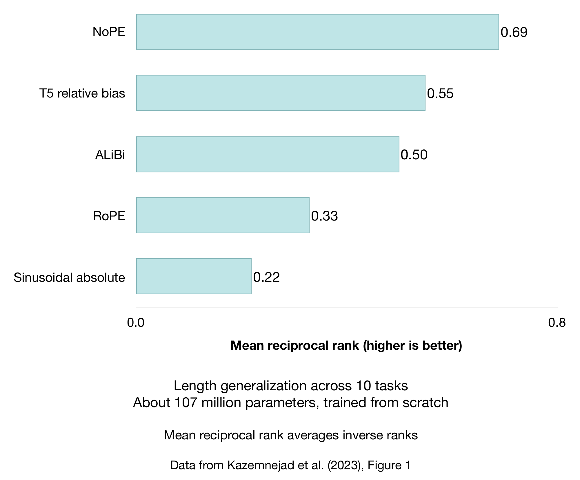
NoPE achieved a mean reciprocal rank of 0.69, compared with 0.55 for T5 relative bias and 0.33 for RoPE. This metric averages inverse method ranks, so higher is better. These values are ranking scores, not accuracy percentages. The absolute baseline in this comparison uses fixed sinusoidal embeddings.
These results show that explicit positional encodings aren’t required for these causal models to learn useful position information. But note that they don’t establish that NoPE will outperform RoPE in every LLM, and I think there is a reason why teams mix RoPE and NoPE layers versus relying on just NoPE everywhere.
Furthermore, the paper’s larger code-model experiments in Appendix F also show that NoPE can fail at sufficiently long contexts. (And these experiments train models with their chosen positional method from the start; they don’t test removing RoPE from an already trained model.)
Appendix D. Longer contexts and YaRN
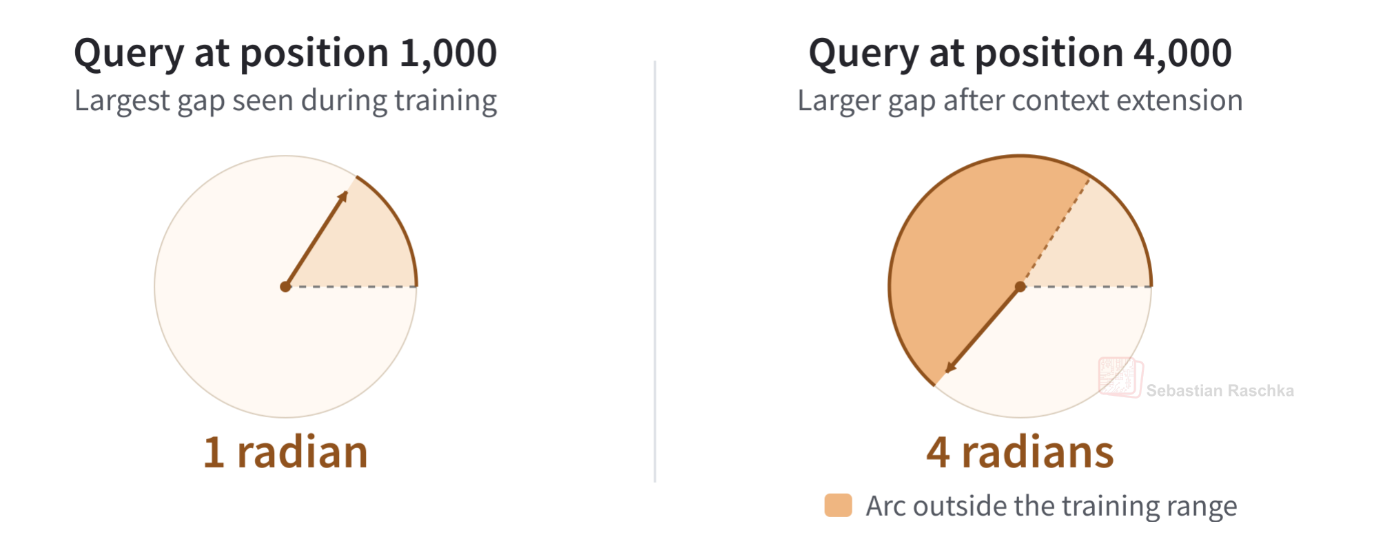
What happens when we the models works with longer documents that result in token gaps much larger than the ones it saw during training? Suppose our model saw gaps of up to 1,000 positions during training. But now, at inference, the query and key might be 4,000 positions apart. Figure D.1 shows what this means for one feature pair that rotates by 0.001 radians per position.

With the key at position 0, the largest relative rotation this pair saw during training was \(1{,}000 \times 0.001 = 1\) radian (left subpanel). If we move the query to position 4,000 the relative rotation becomes \(4{,}000 \times 0.001 = 4\) radians. The orange arc in the right subpanel in the figure above shows how far that takes the pair beyond the angles it saw during training.
Which pair are we looking at in Figure D.1? Figure D.2 shows how the eight entries in the query form four pairs in the 8-feature example from the article. We pair the entries in the key the same way.

How does YaRN decide which pairs to slow down? It considers the number of turns each pair made over the original training context. For instance, over 1,000 positions, the slowest pair (entries 4 and 8) covered just 1 radian, about a sixth of a turn. To extend the context fourfold, YaRN divides this pair’s frequency by four. At 0.00025 radians per position, a gap of 4,000 positions gives it the same 1-radian rotation it saw at a gap of 1,000.
The fastest pair (entries 1 and 5) went around the circle about 159 times. Longer gaps take that fast pair around the circle again. YaRN keeps its frequency, so neighboring positions are still 1 radian apart for that pair.
What about the second-slowest pair (entries 3 and 7)? At 0.01 radians per position, it covered 10 radians, or about 1.6 turns. In their Llama experiments, the YaRN authors used two cutoffs. Pairs below one turn got the full slowdown, pairs above 32 turns kept their frequency, and pairs in between got a partial slowdown. So in our example, both this pair and the next faster pair (entries 2 and 6, about 16 turns) get a partial slowdown.
D.1 How much does YaRN slow down each pair?
As discussed, earlier, the last pair (entries 4 and 8) got the full fourfold slowdown as the slowest pair, so their frequency drops from 0.001 to 0.00025 radians per position.
Now let’s work out the partial slowdown for the second slowest pair (entries 3 and 7). Their original frequency is 0.01 radians per position, and dividing it by four would give us 0.0025. YaRN takes a weighted average of those two frequencies.