• From lecture notes from the STAT479: Machine Learning class I am teaching at UW-Madison

Machine Learning – The Big Picture

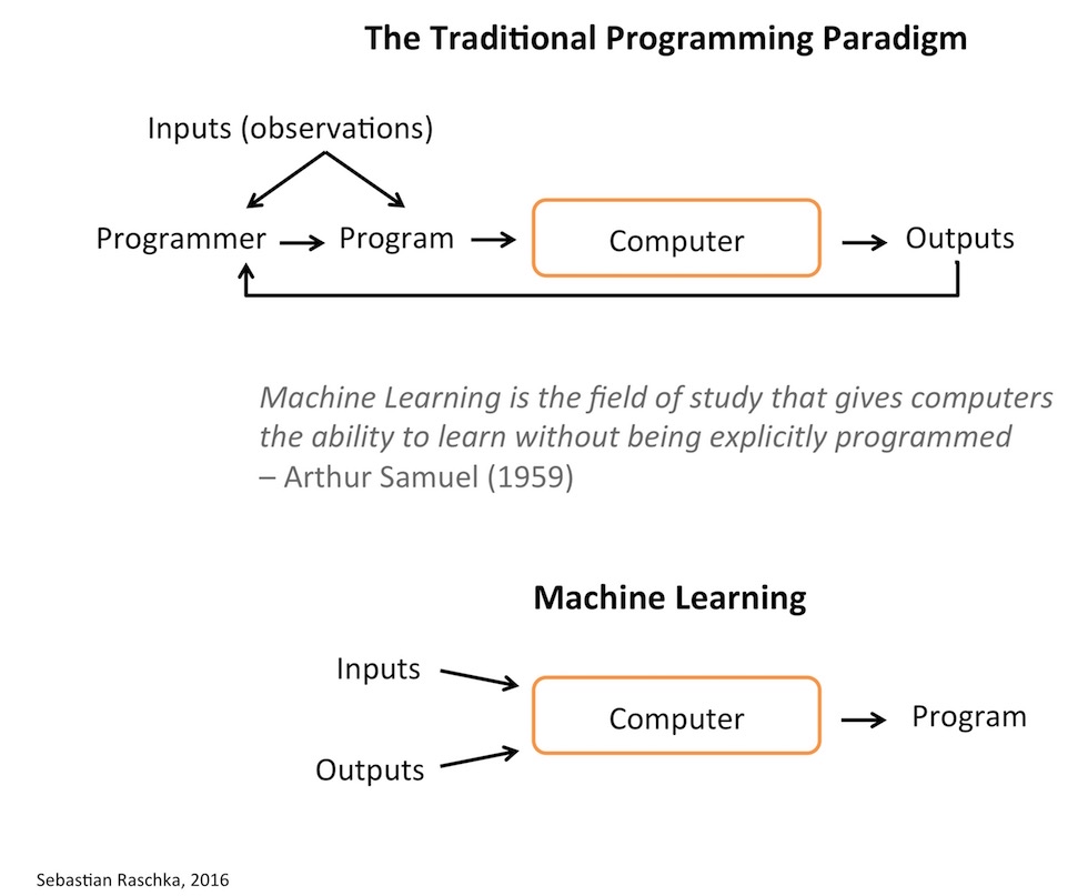
One of the main motivations why we develop (computer) programs to automate various kinds of processes. Originally developed as a subfield of Artificial Intelligence (AI), one of the goals behind machine learning was to replace the need for developing computer programs “manually.” Considering that programs are being developed to automate processes, we can think of machine learning as the process of “automating automation.” In other words, machine learning lets computers “create” programs (often, the intent for developing these programs is making predictions) themselves. In other words, machine learning is the process of turning data into programs.

It is said that the term machine learning was first coined by Arthur Lee Samuel, a pioneer in the AI field, in 1959 \footcite{samuel1959some}. One quote that almost every introductory machine learning resource cites is the following, which summarizes the concept behind machine learning nicely and concisely:

Machine learning is the field of study that gives computers the ability to learn without being explicitly programmed. \footnote{This is not a direct quote but a paraphrased version of Samuel’s sentence “Programming computers to learn from experience should eventually eliminate the need for much of this detailed programming effort.”} — Arthur L. Samuel, AI pioneer, 1959

Now, before we introduce machine learning more formally, here is what some other people said about the field:

The field of machine learning is concerned with the question of how to construct computer programs that automatically improve with experience.
— Tom Mitchell, Professor Machine Learning at Carnegie Mellon University and author of the popular “Machine Learning” textbook

Machine learning is the hot new thing.
— John L. Hennessy, President of Stanford (2000–2016)

A breakthrough in machine learning would be worth ten Microsofts.
— Bill Gates, Microsoft Co-Founder

{ width=65% }

A bit more concrete is Tom Mitchell’s description from his Machine Learning book \footcite{mitchell1997machine}:

A computer program is said to learn from experience \(E\) with respect to some class of tasks \(T\) and performance measure \(P\), if its performance at tasks in \(T\), as measured by \(P\), improves with experience \(E\).
— Tom Mitchell, Machine Learning Professor at Carnegie Mellon University

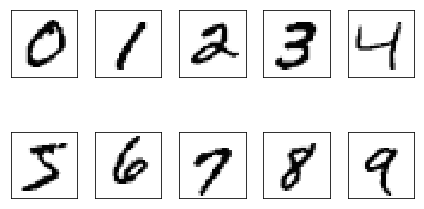
To illustrate this quote with an example, consider the problem of recognizing handwritten digits:

• Task \(T\): classifying handwritten digits from images

• Performance measure \(P\) : percentage of digits classified correctly

• Training experience \(E\): dataset of digits given classifications, e.g., MNIST\footcite{lecun1998gradient}

{ width=50% }

Applications of Machine Learning

After the field of machine learning was “founded” more than a half a century ago, we can now find applications of machine learning in almost every aspect of hour life. Popular applications of machine learning include the following:

• Email spam detection

• Face detection and matching (e.g., iPhone X)

• Web search (e.g., DuckDuckGo, Bing, Google)

• Sports predictions

• Post office (e.g., sorting letters by zip codes)

• ATMs (e.g., reading checks)

• Credit card fraud

• Stock predictions

• Smart assistants (Apple Siri, Amazon Alexa, …)

• Product recommendations (e.g., Netflix, Amazon)

• Self-driving cars (e.g., Uber, Tesla)

• Language translation (Google translate)

• Sentiment analysis

• Drug design

• Medical diagnoses

• …

While we go over some of these applications in class, it is a good exercise to think about how machine learning could be applied in these problem areas or tasks listed above:

• What is the desired outcome?
• What could the dataset look like?
• Is this a supervised or unsupervised problem, and what algorithms would you use? (Something to revisit later in this semester.)
• How would you measure success?
• What are potential challenges or pitfalls?

Overview of the Categories of Machine Learning

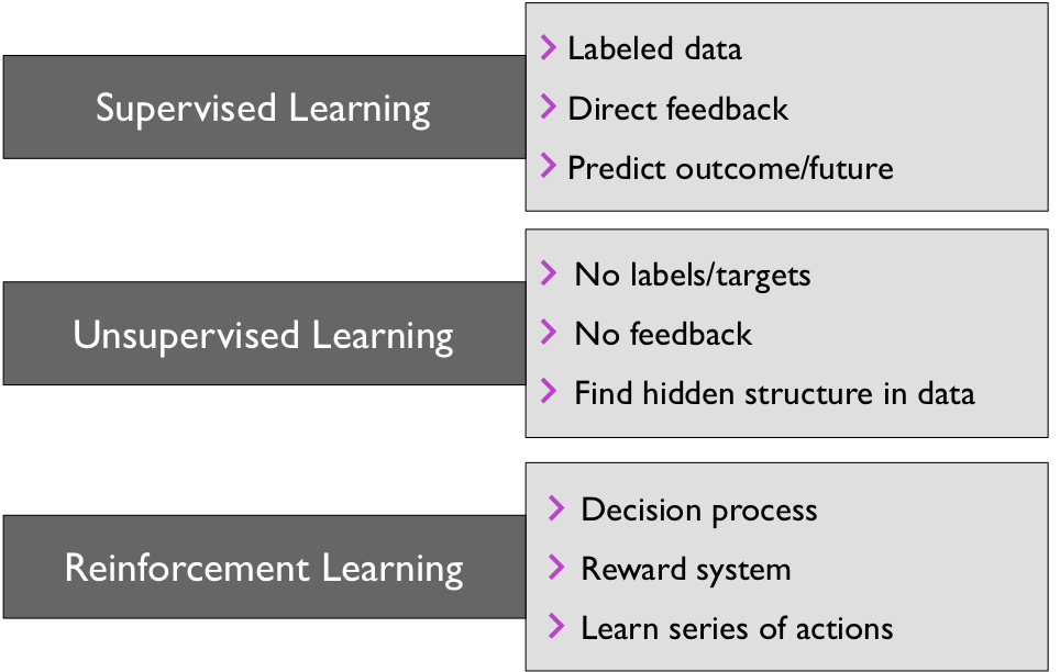
The three broad categories of machine learning are summarized in the following figure: Supervised learing, unsupervised learning, and reinforcement learning. Note that in this class, we will primarily focus on supervised learning, which is the “most developed” branch of machine learning. While we will also cover various unsupervised learning algorithms, reinforcement learning will be out of the scope of this class.

{ width=70% }

Supervised Learning

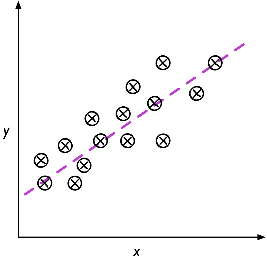
Supervised learning is the subcategory of machine learning that focuses on learning a classification or regression model, that is, learning from labeled training data (i.e., inputs that also contain the desired outputs or targets; basically, “examples” of what we want to predict).

{ width=50% }

{ width=50% }

Unsupervised learning

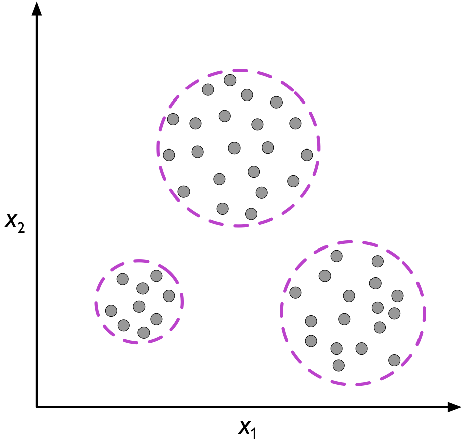
In contrast to supervised learning, unsupervised learning is a branch of machine learning that is concerned with unlabeled data. Common tasks in unsupervised learning are clustering analysis (assigning group memberships) and dimensionality reduction (compressing data onto a lower-dimensional subspace or manifold).

{ width=60% }

Reinforcement learning

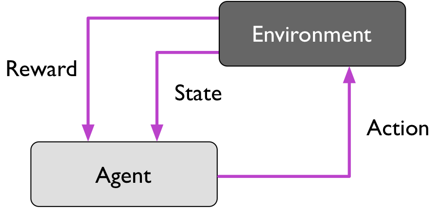
Reinforcement is the process of learning from rewards while performing a series of actions. In reinforcement learning, we do not tell the learner or agent, for example, a (ro)bot, which action to take but merely assign a reward to each action and/or the overall outcome. Instead of having “correct/false” label for each step, the learner must discover or learn a behavior that maximizes the reward for a series of actions. In that sense, it is not a supervised setting and somewhat related to unsupervised learning; however, reinforcement learning really is its own category of machine learning. Reinforcement learning will not be covered further in this class.

Typical applications of reinforcement learning involve playing games (chess, Go, Atari video games) and some form of robots, e.g., drones, warehouse robots, and more recently self-driving cars.

{ width=50% }

Semi-supervised learning

Losely speaking, semi-supervised learning can be described as a mix between supervised and unsupervised learning. In semi-supervised learning tasks, some training examples contain outputs, but some do not. We then use the labeled training subset to label the unlabeled portion of the training set, which we then also utilize for model training.

Introduction to Supervised Learning

Unless noted otherwise (later in future lectures), we will focus on supervised learning and classification, the most prevalent form of machine learning, from now on.

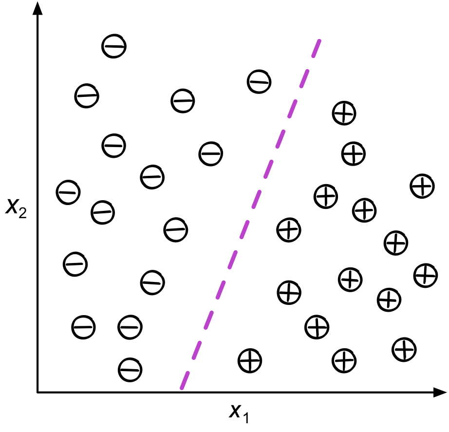
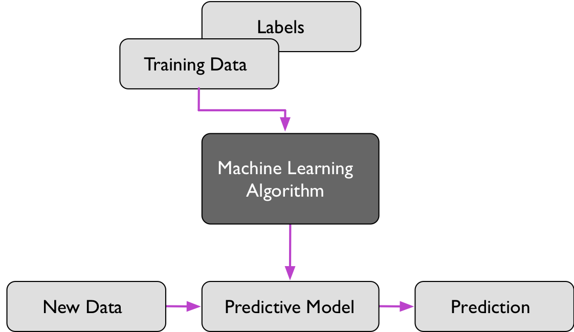
In supervised learning, we are given a labeled training dataset from which a machine learning algorithm can learn a model that can predict labels of unlabeled data points. These unlabeled data points could be either test data points (for which we actually have labels but we withold them for testing purposes) or unlabeled data we will collect in future. For example, given a corpus of spam and non-spam email, a supervised learning task would be to learn a model that predicts to which class (spam or non-spam) new emails belong.

More formally, we define \(h\) as the “hypothesis,” a function that we use to approximate some unknown function \(f(\mathbf{x}) = y,\) where \(\mathbf{x}\) is a vector of input features associated with a training example or dataset instance (for example, the pixel values of an image) and \(y\) is the outcome we want to predict (e.g., what class of object we see in an image). In other words, \(h(\mathbf{x})\) is a function that predicts \(y\).

In classification, we define the hypothesis function as \(h: \mathcal{X} \rightarrow \mathcal{Y} ,\) where \(\mathcal{X} = \mathbb{R}^m\) and \(\mathcal{Y} = \{1, ..., k\}\) with class labels \(k\). in the special case of binary classification, we have \(\mathcal{Y}=\{0, 1\}\) (or \(\mathcal{Y}=\{-1, 1\}\)).

And in regression, the task is to learn a function \(h: \mathbb{R}^m \rightarrow \mathbb{R}.\) Given a training set \(\mathcal{D} = \{<\mathbf{x}^{[i]}, y^{[i]}>, i=1, \ldots\ , n\},\) we denote the \(i\)th training example as \(<\mathbf{x}^{[i]}, y^{[i]}>\). Please note that the superscript \([i]\) is unrelated to exponentiation, and we choose this rather unconvential notational convention for reasons that will become apparent later in this lecture. Note that a critical assumption for (most) machine learning theory is that the training examples are i.i.d. (independent and indentically distributed).

{ width=65% }

{ width=70% }

A crucial assumption we make in supervised learning is that the training examples have the same distribution as the test (future) examples. In real-world applications, this assumption is oftentimes violated, which is one of the common challenges in the field.

Statistical Learning Notation

Please note that the notation varies wildly across the literature, since machine learning is a field that is popular across so many disciplines. For example, in the context of statistical learning theory, we can think of the dataset \(\mathcal{D} = \{<\mathbf{x}^{[1]}, y^{[1]}>, <\mathbf{x}^{[2]}, y^{[2]}> \ldots\ , <\mathbf{x}^{[n]}, y^{[n]}>\}\) as a sample from the population of all possible input-target pairs, and \(\mathbf{x}^{[i]}\) and \(y^{[i]}\) are instances of two random variables \(X \in \mathcal{X}\) and \(Y \in \mathcal{Y}\) and that the training pairs are drawn from a joint distribution $$P(X, Y) = P(X) P(Y

X)$$.

Given an error term \(\epsilon\) we can then formulate the following relationship:

\(Y= f(X) + \epsilon.\) The goal in statistical learning is then to estimate \(f\), which can then be used to predict \(Y\):

\[\hat{f}(X) = \hat{Y}.\]

Data Representation and Mathematical Notation

In previous section, we defined refered to the \(i\)th pair in a labeled training set \(\mathcal{D}\) as \(<\mathbf{x}^{[i]}, y^{[i]}>\).

We will adopt the convention to use italics for scalars, boldface characters for vectors, and uppercase boldface fonts for matrices.

• \(x\): A scalar denoting a single training example with 1 feature (e.g., the height of a person)
• \(\mathbf{x}\): A training example with \(m\) features (e.g,. with \(m=3\) we could represent the height, weight, and age of a person), represented as a column vector (i.e., a matrix with 1 column, \(\mathbf{x} \in \mathbb{R}^{m}\)),

\[\mathbf{x} = \begin{bmatrix} x_1 \\ x_2 \\ \vdots \\ x_m \end{bmatrix}.\]

(Note that most programming languages, incl. Python, start indexing at 0!)

• \(\mathbf{X}\): Design matrix, \(\mathbf{X} \in \mathbb{R}^{n \times m}\), which stores \(n\) training examples, where \(m\) is the number of features.

\(\mathbf{X} = \begin{bmatrix} \mathbf{x}^T_1 \\ \mathbf{x}^T_2 \\ \vdots \\ \mathbf{x}^T_n \end{bmatrix}.\) Note that in order to distinguish the feature index and the training example index, we will use a square-bracket superscript notation to refer to the \(i\)th training example and a regular subscript notation to refer to the \(j\)th feature:

\[\mathbf{X} = \begin{bmatrix} x^{[1]}_{1} & x^{[1]}_{2} & \cdots & x_m^{[1]} \\ x^{[2]}_{1} & x^{[2]}_{2}& \cdots & x_m^{[2]} \\ \vdots & \vdots & \ddots & \vdots \\ x_1^{[n]} & x_2^{[n]} & \cdots & x_m^{[n]} \end{bmatrix}.\]

The corresponding targets are represented in a column vector \(\mathbf{y}, \quad \mathbf{y} \in \mathbb{R}^{n}\) : \(\mathbf{y} = \begin{bmatrix} y^{[1]} \\ y^{[2]} \\ \vdots \\ y^{[n]} \end{bmatrix}.\)

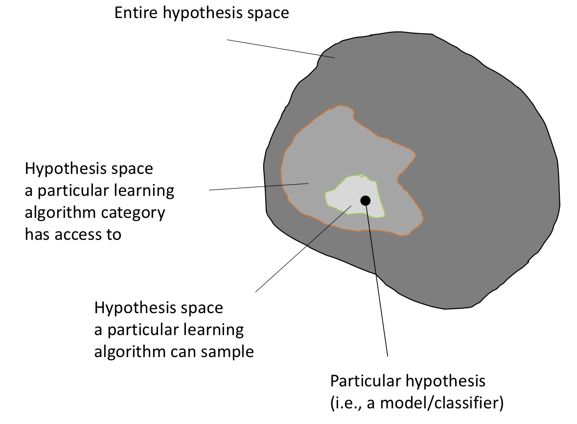
Hypothesis space

In the previous section on supervised learning, we defined the hypothesis \(h(\mathbf{x})\) to predict a target \(y\). Machine learning algorithms sample from a hypothesis space that is usually smaller than the entire space of all possible hypotheses \(\mathcal{H}\) – an exhaustive search covering all \(h \in \mathcal{H}\) would be computationally infeasible since \(\mathcal{H}\) grows exponentially with the size (dimensionality) of the training set. This is illustrated in the following paragraph.

Assume we are given a dataset with 4 features and 3 class labels, the class label (\(y \in \{ \text{Setosa}, \text{Versicolor}, \text{Virginica}\}\)). Also, assume all features are binary. Given 4 features with binary values (True, False), we have \(2^4=16\) different feature combinations (see table below). Now, of the 16 rules, we have three classes to consider (Setosa, Versicolor, Virginica). Hence, we have \(3^{16} = 43,046,721\) potential combinations of 16 rules that we can evaluate (this is the size hypothesis space, $$

\mathcal{H}

=43,046,721$$)!

sepal length \textless 5 cm	sepal width \textless 5 cm	petal length \textless 5 cm	petal width \textless 5 cm	Class Label
True	True	True	True	Setosa
True	True	True	False	Versicolor
True	True	False	True	Setosa
…	…	…	…

Table: Example of decision rules for the Iris flower data dataset.

Now, imagine the features are not binary but real-valued. The hypothesis space will become so big that it would be impossible to evaluate it exhaustively. Hence, we use machine learning to reduce the search space within the hypothesis space. (A neural network with a single hidden layer, a finite number of neurons, and non-linear activation functions such as sigmoid units, was proved to be a universal function approximator \footcite{cybenko1989approximations}. However, the concept of universal function approximation \footcite{csaji2001approximation} does not imply practicality, usefulness, or adequate performance in practical problems.

{ width=70% }

Typically, the number of training examples required is proportional to the flexibility of the learning algorithms. I.e., we need more training for models with

• a large number of parameters to fit;
• a large number of “knobs” to tune (hyperparameters);
• a large size of the hypothesis set to select from.

(As a rule of thumb, the more parameter to fit and/or hyperparameters to tune, the larger the set of hypotheses to choose from).

Classes of Machine Learning Algorithms

Below are some classes of algorithms that were are going to discuss in this class:

• Generalized linear models (e.g., logistic regression)

• Support vector machines (e.g., linear SVM, RBF-kernel SVM)

• Artificial neural networks (e.g., multi-layer perceptrons)

• Tree- or rule-based models (e.g., decision trees)

• Graphical models (e.g., Bayesian networks)

• Ensembles (e.g., Random Forest)

• Instance-based learners (e.g., K-nearest neighbors)

Algorithm Categorization Schemes

To aid our conceptual understsanding, each of the algorithms can be categorized into various categories.

• eager vs lazy;
• batch vs online;
• parametric vs nonparametric;
• discriminative vs generative.

These concepts or categorizations will become more clear once we discussed a few of the different algorithms. However, below are brief descriptions of the various categorizations listed above.

Eager vs lazy learners. Eager learners are algorithms that process training data immediately whereas lazy learners defer the processing step until the prediction. In fact, lazy learners do not have an explicit training step other than storing the training data. A popular example of a lazy learner is the Nearest Neighbor algorithm, which we will discuss in the next lecture.

Batch vs online learning. Batch learning refers to the fact that the model is learned on the entire set of training examples. Online learners, in contrast, learn from one training example at the time. It is not uncommon, in practical applications, to learn a model via batch learning and then update it later using online learning.

Parametric vs nonparametric models. Parametric models are “fixed” models, where we assume a certain functional form for \(f(\mathbf{x})=y\). For example, linear regression can be considered as a parametric model with \(h(\mathbf{x}) = w_1x_1 + ... +w_mx_m + b\). Nonparametric models are more “flexible” and do not have a pre-specfied number of parameters. In fact, the number of parameters grows typically with the size of the training set. For example, a decision tree would be an example of a nonparametric model, where each decision node (e.g., a binary “True/False” assertion) can be regarded as a parameter.

Discriminative vs generative. Generative models (classically) describe methods that model the joint distribution

\[P(X, Y) = P(Y) P(X|Y) = P(X) P(Y|X)\]

for training pairs

\[\langle \mathbf{x}^{[i]}, y^{[i]} \rangle.\]

\footnote{However, in recent years, the term “generative model” has also been used to describe models that learn an approximation of \(X\) and sample training examples \(\mathbf{x} \sim X\). Examples of such models are Generative Adversarial Networks and Variational Autoencoders; deep learning models that are not covered in this class.}.

Discriminative models are taking a more “direct” approach for modeling \(P(Y|X)\) directly. While generative models provide typically more insights and allow sampling from the joint distribution, discriminative models are typically easier to compute and produce more accurate predictions. Helpful for understanding discriminative models is the following analogy: discriminative modeling is like trying to extract information from text in a foreign language without learning that language.

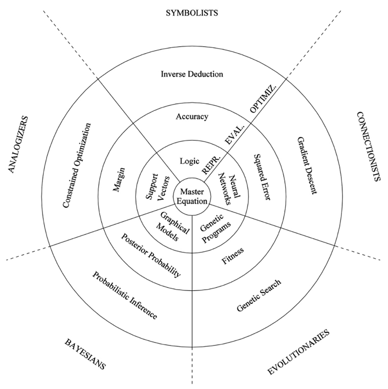
Pedro Domingo’s 5 Tribes of Machine Learning

Another useful way to think about different machine learning algorithms is Pedro Domingons categorization of machine learning algorithms into five tribes, which he defined in his book “The Master Algorithm” \footcite{domingos2015master}.

• Evolutionaries: e.g., genetic algorithms
• Eonnectionists: e.g., neural networks
• Symbolists: e.g., logic
• Bayesians: e.g., graphical models
• Analogizers: e.g., support vector machines

{ width=70% }

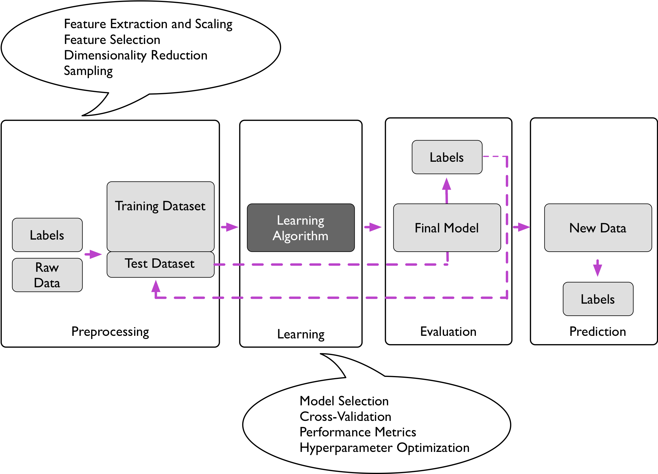
Components of Machine Learning Algorithms

As it was already indicated in the figure of Pedro Domingo’s 5 Tribes of Machine Learning, there are several different components of machine learning algorithms.

Representation. The first component is the “representation,” i.e., which hypotheses we can represent given a certain algorithm class.

Optimization. The second component is the optimization metric that we use to fit the model.

Evaluation. The evaluation component is the step where we evaluate the performance of the model after model fitting.

To extend this list slightly, these are the following 5 steps that we want to think about when approaching a machine learning application:

1. Define the problem to be solved.
2. Collect (labeled) data.
3. Choose an algorithm class.
4. Choose an optimization metric for learning the model.
5. Choose a metric for evaluating the model.

Note that optimization objectives are usually not the same in practice. For example, the optimization objective of the logistic regression algorithm is to minimize the negative log-likelihood (or binary cross-entropy), whereas the evaluation metric could be the classification accuracy or misclassification error.

Also, while the list above indicates a linear workflow, in practice, we often jump back to previous steps and e.g., collect more data, try out different algorithms, and/or tune the “knobs” (i.e., “hyperparameters”) of learning algorithms.

The following two subsections will provide a short overview of the optimization (training) and evaluation parts.

Training

Training/fitting a classification or regression model typically involves the use of an optimization algorithms that optimizes an objective function (e.g., maximizing the log-likelihood or minimizing mean squared error). Some of the methods that we will cover in this course are the following:

• Combinatorial search, greedy search (e.g., decision trees over, not within nodes);
• Unconstrained convex optimization (e.g., logistic regression);
• Constrained convex optimization (e.g., SVM);
• Nonconvex optimization, here: using backpropagation, chain rule, reverse autodiff. (e.g., neural networks).
• Constrained nonconvex optimization (semi adversarial networks \footcite{mirjalili2018semi}, not covered in this course)

There exists a number of different algorithms for each optimization task category (for example, gradient descent or conjugate gradient, and quasi-Newton methods to optimize convex optimization problems). Also, the objective functions that we optimize can take different forms. Below are some examples:

• Maximize the posterior probabilities (e.g., naive Bayes)
• Maximize a fitness function (genetic programming)
• Maximize the total reward/value function (reinforcement learning)
• Maximize information gain/minimize child node impurities (CART decision tree classification)
• Minimize a mean squared error cost (or loss) function (CART, decision tree regression, linear regression, adaptive linear neurons, …)
• Maximize log-likelihood or minimize cross-entropy loss (or cost) function
• Minimize hinge loss (support vector machine)

Evaluation

Intuition

There are several different evaluation metric to assess the performance of a model, and the most common ones will be discussed in future lectures. Unless noted otherwise, though, we will focus on the classification accuracy (\(\text{ACC}\)) or misclassification error (\(\text{ERR} = 1 - \text{ACC}\)).

The classification accuracy of an algorithm is usually evaluated empirically by counting the fraction of correctly classified instances considering all instances that the model attempted to classify. For instance, if we have a test dataset of 100 instances and a model classified 7,000 out of 10,000 instances correctly, then we say that the model has a 70% accuracy on that dataset. In practice, we are often interested in the generalization performance of a model, which is the performance on new, unseen data that has the same distribution as the training data. The simplest way to estimate the generalization accuracy is to compute the accuracy on a reasonably sized unseen dataset (e.g., the test dataset that we set aside). However, there are several different techniques to estimate the generalization performance which have different strengths and weaknesses. Being such an important topic, we will devote a seperate lecture to model evaluation.

Prediction Error

To introduce the notion of the prediction or misclassification error more formally, consider the 0-1 loss function

\[L(\hat{y}, y) = \begin{cases} 0 &\text{if } \hat{y} = y \\\\ 1 &\text{if } \hat{y} \neq y, \end{cases}\]

where \(\hat{y}\) is the class label predicted by a given hypothesis \(h(\mathbf{x})=\hat{y}\), and \(y\) is the ground truth (correct class label). Then, the prediction error can be defined as the expected value

\[ERR = {\text{E}} \big[L(\hat{Y}, Y)\big],\]

which we can estimate from the test dataset \(\mathcal{D}_\text{test}\):

\[ERR_{\mathcal{D}_\text{test}} = \frac{1}{n} \sum_{i=1}^{n} L\Big(\hat{y}^{[i]}, y^{[i]}\Big),\]

where \(n\) is the number of examples in the test dataset, $$n =

D_{\text{test}}

$$.

As mentioned before, there are many, many more metrics, which can be more useful in specialized contexts, which will be discussed in future lectures. Some of the most popular metrics are:

• Accuracy (1-Error)
• ROC AUC
• Precision
• Recall
• (Cross) Entropy
• Likelihood
• Squared Error/MSE
• L-norms
• Utility
• Fitness
• …

But more on other metrics in future lectures.

Different Motivations for Studying Machine Learning

There are several different motivations or approaches we take when are studying ML. While the following bullet points attempt an overall categorization, there are many exceptions:

• Engineers: Focus on developing systems with high predictive performance for real-world problem solving
• Mathematicians, computer scientists, and statisticians: understanding properties of predictive models and modeling approaches
• Neuroscientists: understanding and modeling how a brain and intelligence works

Note that machine learning was originally inspired by neuroscience, when the first attempt of an artificial neuron, the McCulloch-Pitts Neuron \footcite{mcculloch1943logical}, was modeled after a biological neuron and letter lead to the popular perceptron algorithm by Frank Rosenblatt \footcite{rosenblatt1957perceptron} – more on that in later lectures.

On Black Boxes & Interpretability

As mentioned in earlier section, when we are applying machine learning to real-world problem solving, we need to define the overall objective first and then choose the right tool for the task. Unfortunately, as a rule of thumb, simpler models are usually associated with lower accuracy. Hence, when we are choosing modeling approaches or learning algorithms, we have to think about whether the emphasis is on understanding a phenomenon or making accurate predictions. Then, the problem becomes how meaningful the insights into a modeling procedure are if the predictions are not accurate. (I.e., what is it good for if I understand the model if the model is wrong).

In this context, a famous quote by our department’s founder:

All models are wrong; some models are useful.
— George Box (1919-2013), Professor of Statistics at UW-Madison

{ width=25% }

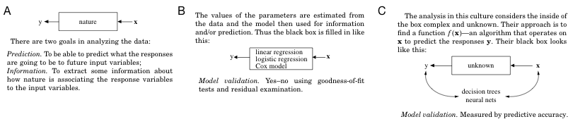
Back in 2001, Leo Breiman wrote an interesting, highly recommended article called “Statistical Modeling: The Two Cultures” \footcite{breiman2001statistical} where he contrasted two different approaches with respect the the two different goals “information” and “prediction.” He referred to the two approaches as the “data modeling culture” and the “algorithmic modeling culture.”

{ width=90% }

The moral of the story is that whether to choose a “data model” or an “algorithmic model” really depends on the problem we want to solve, and it’s best to use the appropriate tool for the task. In this course, we will of course not be restricted to one kind or the other. We will cover techniques of what would fit into the “data modeling culture” (Bayes optimal classifiers, Bayesian networks, naive Bayes, logistic regression, etc.) as well as “algorithmic approaches” (k-nearest neighbors, decision trees, support vector machines, etc.).

Further, Breiman mentions three lessons learned in the statistical modeling and machine learning communities, which I summarized below:

• Rashomon effect; the the multiplicity of good models. Often we have mutliple good models that fit the data well. If we have different models that all fit the data well, which one should we pick?
• Occam’s razor. While we prefer favoring simple models, there is usually a conflict between accuracy and simplicity to varying degree (in later lectures, we will learn about techniques for selecting models within a “sweet spot” considering that this is a trade-off)
• Bellman and the “curse of dimensionality.” Usually, having more data is considered a good thing (i.e., more information). However, more data can be harmful to a model and make it more prone to overfitting (fitting the training data too closely and not generalizing well to new data that was not seen during training; fitting noise). Note that the curse of dimensionality refers to an increasing number of feature variables given a fixed number of training examples. Some models have smart workarounds for dealing with large feature sets. E.g., Breiman’s random forest algorithm, which partitions the feature space to fit individual decision trees that are then later joined to a decistion tree ensemble (the particular algorithm is called random forest), but more on that in future lectures.

Also note that there’s a “No Free Lunch” theorem for machine learning \footcite{wolpert1996lack}, meaning that there’s no single best algorithm that works well across different problem domains.

The Relationship between Machine Learning and Other Fields

Machine Learning and Data Mining

Data mining focuses on the discovery of patterns in datasets or “gaining knowledge and insights” from data – often, this involves a heavy focus on computational techniques, working with databases, etc (nowdays, the term is more or less synonymous to “data science”). We can then think of machine learning algorithms as tools within a data mining project. Data mining is not “just” but also emphasis data processing, visualization, and tasks that are traditionally not categorized as “machine learning” (for example, association rule mining).

Machine Learning, AI, and Deep Learning

Artificial intelligence (AI) was created as a subfield of computer science focussing on solving tasks that humans are good at (for example, natural language processing, image recognition). Or in other words, the goal of AI is to mimick human intelligence.

There are two subtypes of AI: Artificial general intelligence (AGI) and narrow AI. AGI refers to an intelligence that equals humans in several tasks, i.e., multi-purpose AI. In contrast, narrow AI is more narrowly focused on solving a particular task that humans are traditionally good at (e.g., playing a game, or driving a car – I would not go so far and refer to “image classification” as AI).

In general, AI can be approached in many ways. One approach is to write a computer program that implements a set of rules devised by domain experts. Now, hand-crafting rules can be very laborious and time consuming. The field of machine learning then emerged as a subfield of AI – it was concerned with the development of algorithms so that computers can automatically learn (predictive) models from data.

Assume we want to develop a program that can recognize handwritten digits from images. One approach would be to look at all of these images and come up with a set of (nested) if-this-than-that rules to determine which digit is displayed in a particular image (for instance, by looking at the relative locations of pixels). Another approach would be to use a machine learning algorithm, which can fit a predictive model based on a thousands of labeled image samples that we may have collected in a database.

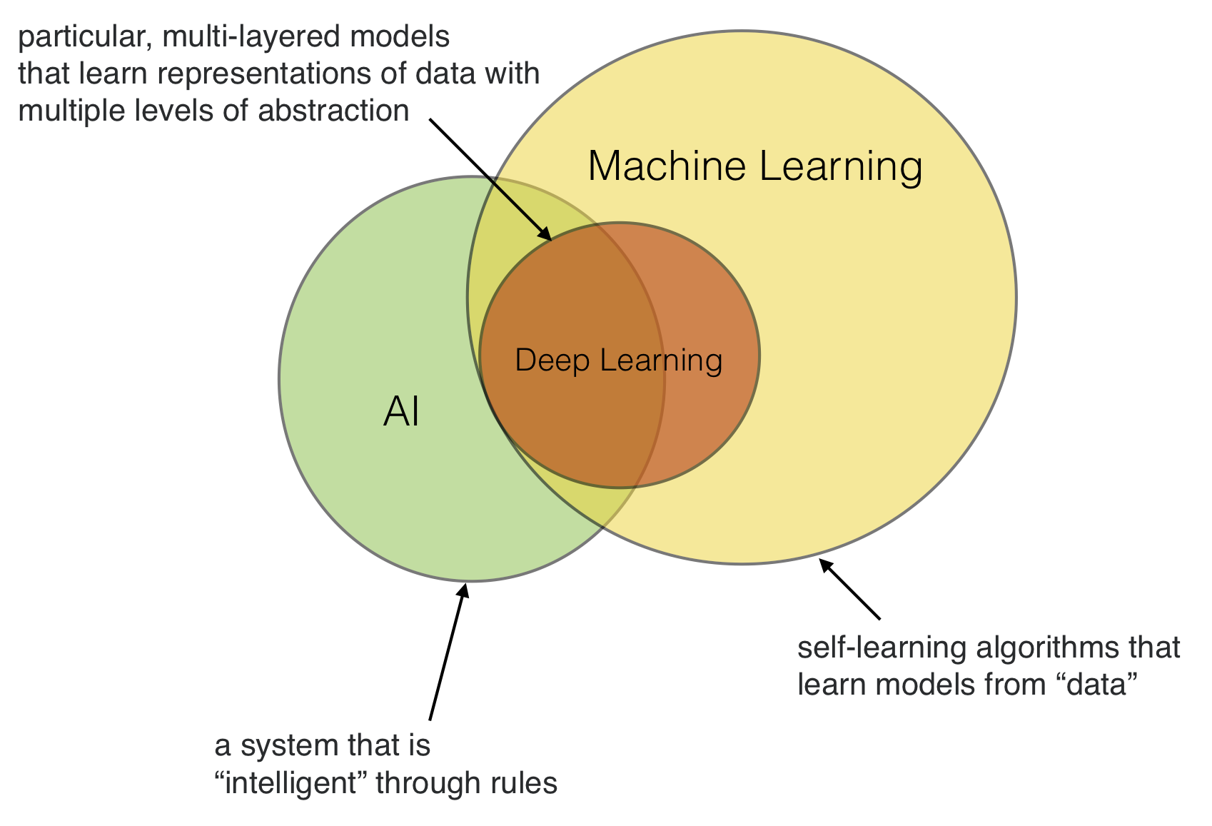
Now, there is also deep learning, which in turn is a subfield of machine learning, referring to a particular subset of models that are particularly good at certain tasks such as image recognition and natural language processing. We will talk more about deep learning toward the end of this class.

Or in short, machine learning (and deep learning) definitely helps to develop “AI,” however, AI doesn’t necessarily have to be developed using machine learning – although, machine learning makes “AI” much more convenient.

{ width=80% }

Roadmap for this Course

This is an outline that might change depending on how the course progresses. If we have to skip the deep learning part, that’s okay. There will be a whole course dedicated to deep learning offered in future.

Date	Description
Part I: Introduction
	Course Overview, Intro to ML
	Intro to Supervised Learning: KNN
Part II: Computational Foundations
	Python, Matplotlib, Jupyter Notebooks
	NumPy, SciPy, Scikit-Learn
	Data Preprocessing
Part III: Tree-Based Methods
	Decision Trees
	Ensemble Methods
Part IV: Evaluation
	Model Selection & Evaluation 1
	Model Selection & Evaluation 2
Part V: Dimensionality Reduction
	Feature Selection
	Feature Extraction
Part V: Bayesian Learning
	Bayes Classifiers
	Text Data & Sentiment Analysis
	Naïve Bayes Classification
Part VI: Regression and Unsupervised Learning
	Regression Analysis
	Clustering
Part VII: Artificial Neural Networks
	Perceptron
	Adaline & Logistic Regression
	SVM
	Multilayer Perceptron
Part VIII: Deep Learning
	Intro to TensorFlow, PyTorch
	CNNs (Deep Learning)
	RNNs (Deep Learning)
	Training Neural Nets: “Tricks of the Trade”

Software

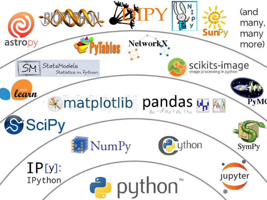
We will talk more about software in upcoming lectures, but at this point, I want to provide a brief overview of the “Python for scientific computing” landscape.

{ width=70% }

The Python-topics we will make use of in this course are the following:

• Python, IPython / Jupyter Notebooks
• NumPy, SciPy, Matplotlib, Scikit-learn, Pandas

Glossary

Machine learning borrows concepts from many other fields and redefines what has been known in other fields under different names. Below is a small glossary of machine learning-specfic terms along with some key concepts to help navigate the machine learning literature.

• Training example: A row in the table representing the dataset. Synonymous to an observation, training record, training instance, training sample (in some contexts, sample refers to a collection of training examples) or simply data point.
• Training: model fitting, for parametric models similar to parameter estimation.
• Feature, \(x\): a column in the table representing the dataset. Synonymous to predictor, variable, input, attribute.
• Target, \(y\): Synonymous to outcome, output, response variable, dependent variable, (class) label, ground truth.
• Predicted output, \(\hat{y}\): use this to distinguish from targets; here, means output from the model.

• Loss function: Often used synomymously with cost function; sometimes also called error function. In some contexts the loss for a single data point, whereas the cost function refers to the overall (average or summed) loss over the entire dataset.

• Hypothesis: A hypothesis is a certain function that we believe (or hope) is similar to the true function, the target function that we want to model. In context of spam classification, it would be a classification rule we came up with that allows us to separate spam from non-spam emails.
• Model: In the machine learning field, the terms hypothesis and model are often used interchangeably. In other sciences, they can have different meanings: A hypothesis could be the “educated guess” by the scientist, and the model would be the manifestation of this guess to test this hypothesis.
• Learning algorithm: Again, our goal is to find or approximate the target function, and the learning algorithm is a set of instructions that tries to model the target function using our training dataset. A learning algorithm comes with a hypothesis space, the set of possible hypotheses it explores to model the unknown target function by formulating the final hypothesis.
• Classifier: A classifier is a special case of a hypothesis (nowadays, often learned by a machine learning algorithm). A classifier is a hypothesis or discrete-valued function that is used to assign (categorical) class labels to particular data points. In an email classification example, this classifier could be a hypothesis for labeling emails as spam or non-spam. Yet, a hypothesis must not necessarily be synonymous to the term classifier. In a different application, our hypothesis could be a function for mapping study time and educational backgrounds of students to their future, continuous-valued, SAT scores – a continuous target variable, suited for regression analysis.
• Hyperparameters: Hyperparameters are the tuning parameters of a machine learning algorithm – for example, the regularization strength of an L2 penalty in the mean squared error cost function of linear regression, or a value for setting the maximum depth of a decision tree. In contrast, model parameters are the parameters that a learning algorithm fits to the training data – the parameters of the model itself. For example, the weight coefficients (or slope) of a linear regression line and its bias (or y-axis intercept) term are model parameters.

Reading Assignments

• Raschka and Mirjalili: Python Machine Learning, 2nd ed., Ch 01
• Trevor Hastie, Robert Tibshirani, and Jerome Friedman: The Elements of Statistical Learning, Ch 01

Further Reading

Optional reading beyond the scope of this class for those who are interested.

• Statistical Modeling: The Two Cultures (2001) by Leo Breiman, https://projecteuclid.org/euclid.ss/1009213726