Latent MoE
Latent MoE is still a sparse MoE, but with the difference that the expert computation no longer happens at the model’s full hidden width.
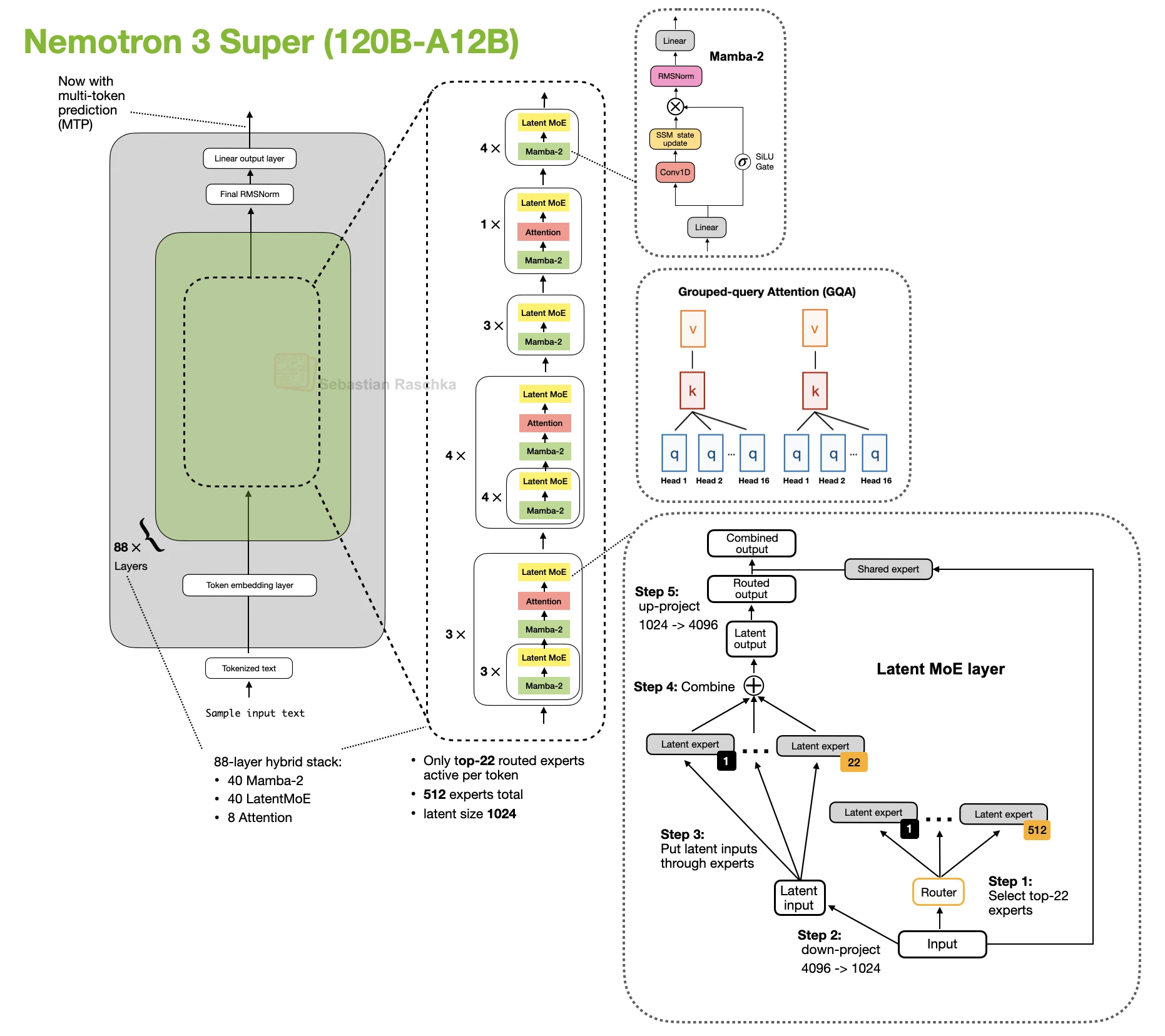
The architecture that introduced it is Nemotron 3 Super. Here, Instead of running the experts directly at width 4096, the model first projects down to 1024, applies the routed experts there, and then projects back up. So the routing idea stays the same, but the expert path itself becomes cheaper (minus the down- and up-projecting overhead).
What changes
The expert path moves into a compressed latent space instead of running at full hidden width
Practical benefit
Lower expert-side compute while keeping the basic sparse-routing setup
Example architecture
Start With Regular MoE
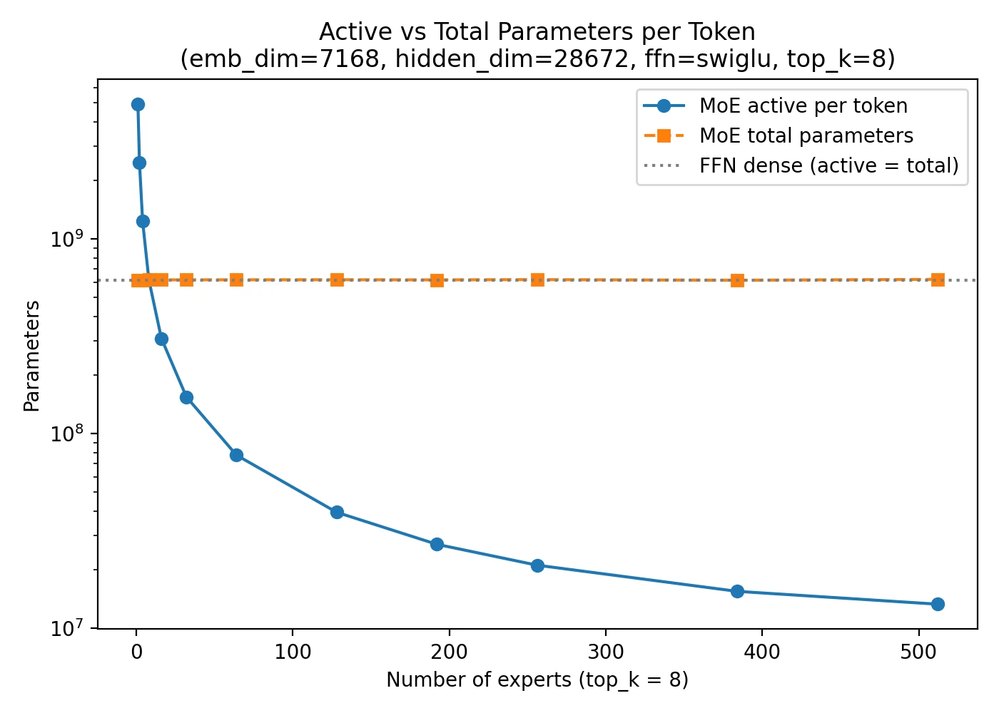
Standard MoE already gives us the large gap between total parameters and active parameters per token. The from-scratch MoE materials are useful here because they make that baseline concrete: the whole point is that the model can be huge in total capacity while activating only a small routed subset on each step.
The Nemotron 3 Super LatentMoE
In LatentMoE, the inputs are down-projected from 4096 to 1024, the experts operate there, and the outputs are then up-projected back to 4096.
That means the model is not only selecting a sparse subset of experts. It is also making each selected expert cheaper to run. This makes latent MoE feel less like a separate MoE family and more like an additional efficiency tweak on top of standard sparse routing.
Example Architectures
- Nemotron 3 Super 120B-A12B: the clearest latent-MoE example in the gallery
- Nemotron 3 Nano 30B-A3B: a useful contrast point because it keeps the broader Nemotron hybrid recipe without the latent-expert change
Sources