Model evaluation, model selection, and algorithm selection in machine learning
Part III - Cross-validation and hyperparameter tuning
A single-PDF version of Model Evaluation parts 1-4 is available on arXiv: https://arxiv.org/abs/1811.12808
Introduction
Almost every machine learning algorithm comes with a large number of settings that we, the machine learning researchers and practitioners, need to specify. These tuning knobs, the so-called hyperparameters, help us control the behavior of machine learning algorithms when optimizing for performance, finding the right balance between bias and variance. Hyperparameter tuning for performance optimization is an art in itself, and there are no hard-and-fast rules that guarantee best performance on a given dataset. In Part I and Part II, we saw different holdout and bootstrap techniques for estimating the generalization performance of a model. We learned about the bias-variance trade-off, and we computed the uncertainty of our estimates. In this third part, we will focus on different methods of cross-validation for model evaluation and model selection. We will use these cross-validation techniques to rank models from several hyperparameter configurations and estimate how well they generalize to independent datasets.
About Hyperparameters and Model Selection
Previously, we used the holdout method or different flavors of bootstrapping to estimate the generalization performance of our predictive models. We split our dataset into two parts: a training and a test dataset. After the machine learning algorithm fit a model to the training set, we evaluated it on the independent test set that we withheld from the machine learning algorithm during model fitting. While we were discussing challenges such as the bias-variance trade-off, we used fixed hyperparameter settings in our learning algorithms, such as the number of k in the K-nearest neighbors algorithm. We defined hyperparameters as the parameters of the learning algorithm itself, which we have to specify a priori — before model fitting. In contrast, we refered to the parameters of our resulting model as the model parameters.
So, what are hyperparameters, exactly? Considering the k-nearest neighbors algorithm, one example of a hyperparameter is the integer value of k. If we set k=3, the k-nearest neighbors algorithm will predict a class label based on a majority vote among the 3-nearest neighbors in the training set. The distance metric for finding these nearest neighbors is yet another hyperparameter of the algorithm.
Now, the k-nearest neighbors algorithm may not be an ideal choice for illustrating the difference between hyperparameters and model parameters, since it is a lazy learner and a nonparametric method. In this context, lazy learning (or instance-based learning) means that there is no training or model fitting stage: A k-nearest neighbors model literally stores or memorizes the training data and uses it only at prediction time. Thus, each training instance represents a parameter in a k-nearest neighbors model. In short, nonparametric models are models that cannot be described by a fixed number of parameters that are being adjusted to the training set. The structure of parametric models is not decided by the training data rather than being set a priori; nonparamtric models do not assume that the data follows certain probability distributions unlike parametric methods (exceptions of nonparametric methods that make such assumptions are Bayesian nonparametric methods). Hence, we may say that nonparametric methods make fewer assumptions about the data than parametric methods.
In contrast to k-nearest neighbors, a simple example of a parametric method would be logistic regression, a generalized linear model with a fixed number of model parameters: a weight coefficient for each feature variable in the dataset plus a bias (or intercept) unit. These weight coefficients in logistic regression, the model parameters, are updated by maximizing a log-likelihood function or minimizing the logistic cost. For fitting a model to the training data, a hyperparameter of a logistic regression algorithm could be the number of iterations or passes over the training set (epochs) in a gradient-based optimization. Another example of a hyperparameter would be the value of a regularization parameter such as the lambda-term in L2-regularized logistic regression:
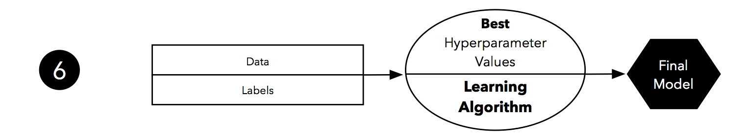
Changing the hyperparameter values when running a learning algorithm over a training set may result in different models. The process of finding the best-performing model from a set of models that were produced by different hyperparameter settings is called model selection. In the next section, we will look at an extension to the holdout method that helps us with this selection process.
The Three-Way Holdout Method for Hyperparameter Tuning
In Part I, we learned that resubstitution validation is a bad approach for estimating of the generalization performance. Since we want to know how well our model generalizes to new data, we used the holdout method to split the dataset into two parts, a training set and an independent test set. Can we use the holdout method for hyperparameter tuning? The answer is “yes!” However, we have to make a slight modification to our initial approach, the “two-way” split, and split the dataset into three parts: a training, a validation, and a test set.
We can regard the process of hyperparameter tuning and model selection as a meta-optimization task. While the learning algorithm optimizes an objective function on the training set (with exception to lazy learners), hyperparameter optimization is yet another task on top of it; here, we typically want to optimize a performance metric such as classification accuracy or the area under a Receiver Operating Characteristic curve. After the tuning stage, selecting a model based on the test set performance seems to be a reasonable approach. However, reusing the test set multiple times would introduce a bias and our final performance estimate and likely result in overly optimistic estimates of the generalization performance — we can say that “the test set leaks information.” To avoid this problem, we could use a three-way split, dividing the dataset into a training, validation, and test dataset. Having a training-validation pair for hyperparameter tuning and model selections allows us to keep the test set “independent” for model evaluation. Now, remember our discussion of the “3 goals” of performance estimation?
- We want to estimate the generalization accuracy, the predictive performance of our model on future (unseen) data.
- We want to increase the predictive performance by tweaking the learning algorithm and selecting the best-performing model from a given hypothesis space.
- We want to identify the machine learning algorithm that is best-suited for the problem at hand; thus, we want to compare different algorithms, selecting the best-performing one as well as the best-performing model from the algorithm’s hypothesis space.
The “three-way holdout method” is one way to tackle points 1 and 2 (more on point 3 in the next article, Part IV). Though, if we are only interested in point 2, selecting the best model, and do not care so much about an “unbiased” estimate of the generalization performance, we could stick to the two-way split for model selection. Thinking back of our discussion about learning curves and pessimistic biases in Part II, we noted that a machine learning algorithm often benefits from more labeled data; the smaller the dataset, the higher the pessimistic bias and the variance — the sensitivity of our model towards the way we partition the data.
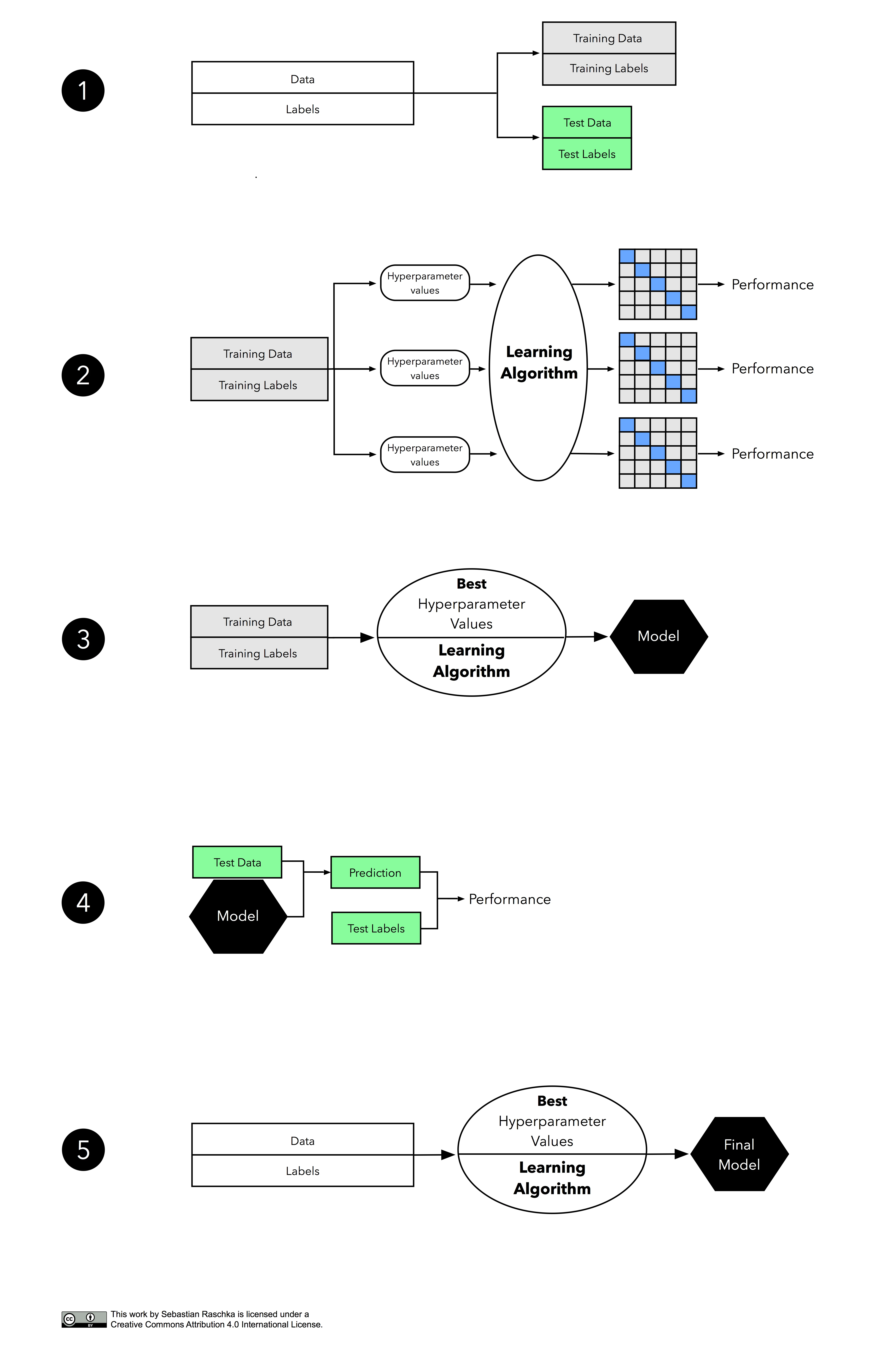
“There ain’t no such thing as a free lunch.” The three-way holdout method for hyperparameter tuning and model selection is not the only — and certainly often not the best — way to approach this task. In later sections, we will learn about alternative methods and discuss their advantages and trade-offs. However, before we move on to the probably most popular method for model selection, k-fold cross-validation (or sometimes also called “rotation estimation” in older literature), let us have a look at an illustration of the 3-way split holdout method:
Since there’s a lot going on in this figure, let’s walk through it step by step.
We start by splitting our dataset into three parts, a training set for model fitting, a validation set for model selection, and a test set for the final evaluation of the selected model.
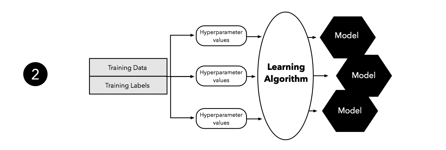
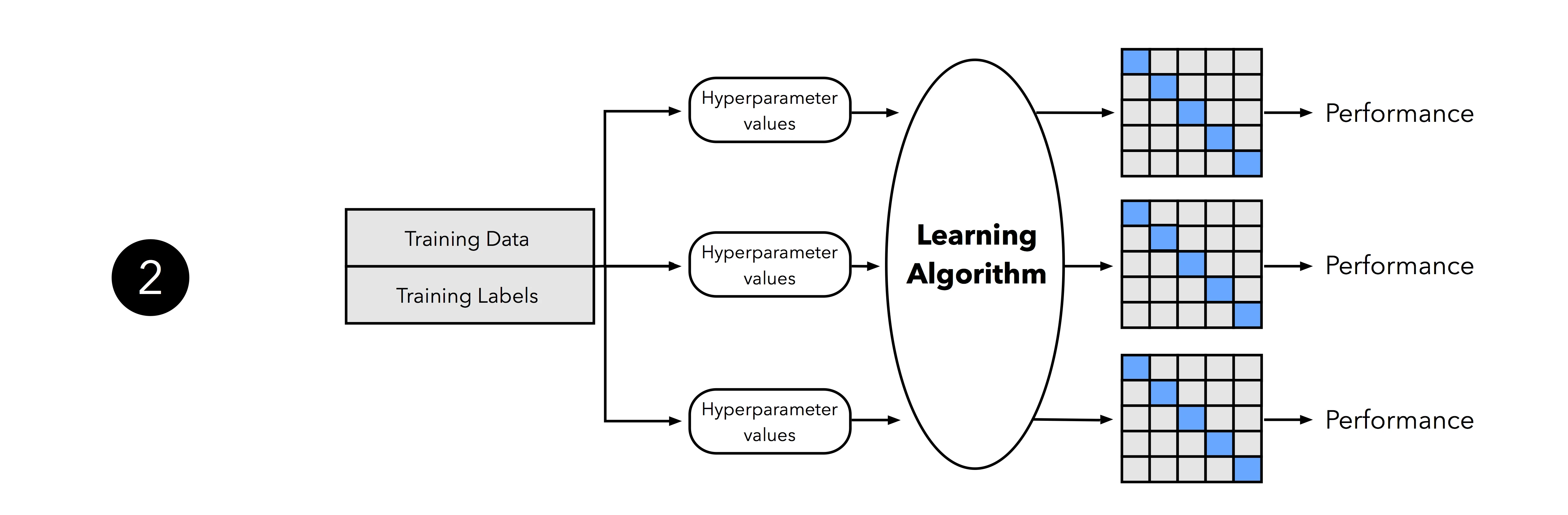
The second step illustrates the hyperparameter tuning stage. We use the learning algorithm with different hyperparameter settings (here: three) to fit models to the training data.
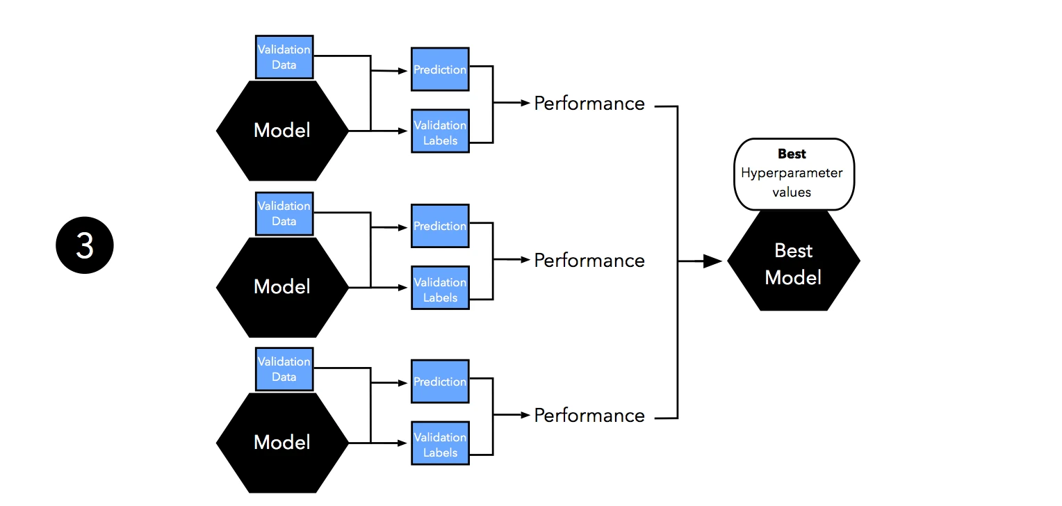
Next, we evaluate the performance of our models on the validation set. This step illustrates the model selection stage; after comparing the performance estimates, we choose the hyperparameters settings associated with the best performance. Note that we often merge steps two and three in practice: we fit a model and compute its performance before moving on to the next model in order to avoid keeping all fitted models in memory.
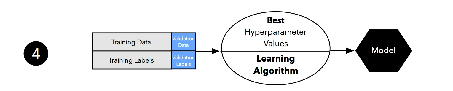
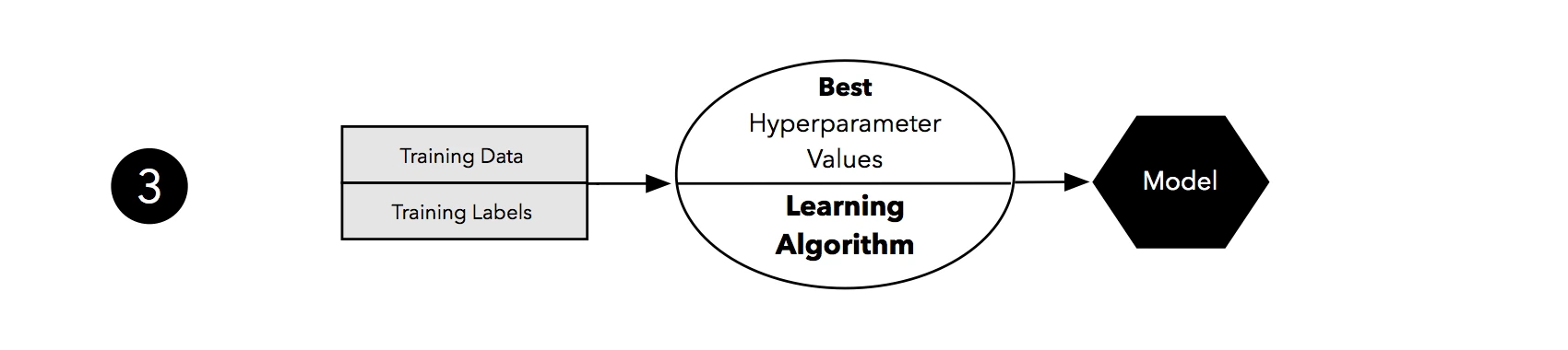
As discussed in Part I and Part II, our estimates may suffer from pessimistic bias if the training set is too small. Thus, we can merge the training and validation set after model selection and use the best hyperparameter settings from the previous step to fit a model to this larger dataset.
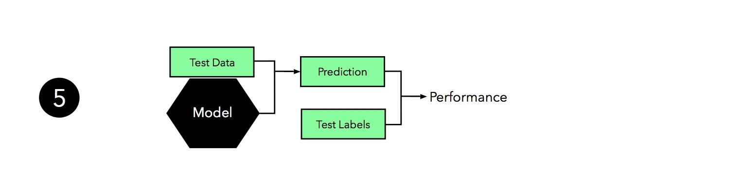
Now, we can use the independent test set to estimate the generalization performance our model. Remember that the purpose of the test set is to simulate new data that the model has not seen before. Re-using this test set may result in an overoptimistic bias in our estimate of the model’s generalization performance.
Finally, we can make use of all our data — merging training and test set — and fit a model to all data points for real-world use.
Note that fitting the model on all available data might yield a model that is likely slightly different from the model evaluated in Step 5. However, in theory, using all data (that is, training and test data) to fit the model should only improve its performance. Under this assumption, the evaluated performance from Step 5 might slightly underestimate the performance of the model fitted in Step 6. (If we use test data for fitting, we do not have data left to evaluate the model, unless we collect new data.) In real-world applications, having the “best possible” model is often desired – or in other words, we do not mind if we slightly underestimated its performance. In any case, we can regard this sixth step as optional.
Introduction to K-fold Cross-Validation
It’s about time to introduce the probably most common technique for model evaluation and model selection in machine learning practice: k-fold cross-validation. The term cross-validation is used loosely in literature, where practitioners and researchers sometimes refer to the train/test holdout method as a cross-validation technique. However, it might make more sense to think of cross-validation as a crossing over of training and validation stages in successive rounds. Here, the main idea behind cross-validation is that each sample in our dataset has the opportunity of being tested. K-fold cross-validation is a special case of cross-validation where we iterate over a dataset set k times. In each round, we split the dataset into k parts: one part is used for validation, and the remaining k-1 parts are merged into a training subset for model evaluation as shown in the figure below, which illustrates the process of 5-fold cross-validation:
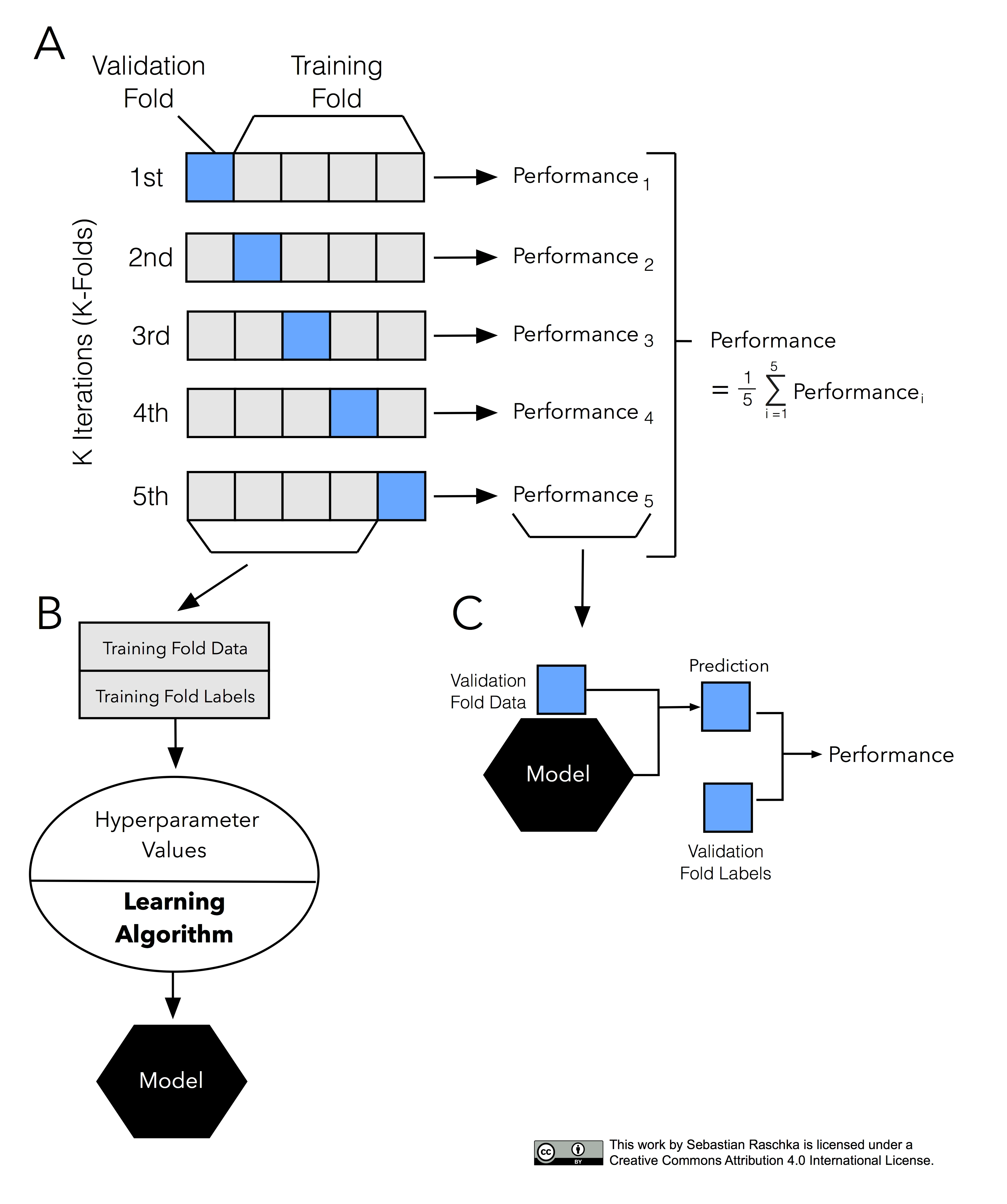
Just as in the “two-way” holdout method, we use a learning algorithm with fixed hyperparameter settings to fit models to the training folds in each iteration — if we use the k-fold cross-validation method for model evaluation. In 5-fold cross-validation, this procedure will result in five different models fitted; these models were fit to distinct yet partly overlapping training sets and evaluated on non-overlapping validation sets. Eventually, we compute the cross-validation performance as the arithmetic mean over the k performance estimates from the validation sets.
We saw the main difference between the “two-way” holdout method and k-fold cross validation: k-fold cross-validation uses all data for training and testing. The idea behind this approach is to reduce the pessimistic bias by using more training data in contrast to setting aside a relatively large portion of the dataset as test data. And in contrast to the repeated holdout method, which we discussed in Part II, test folds in k-fold cross-validation are not overlapping. In repeated holdout, the repeated use of samples for testing results in performance estimates that become dependent between rounds; this dependence can be problematic for statistical comparisons, which we will discuss in Part IV. Also, k-fold cross-validation guarantees that each sample is used for validation in contrast to the repeated holdout-method, where some samples may never be part of the test set.
In this section, we introduced k-fold cross-validation for model evaluation. In practice, however, k-fold cross-validation is more commonly used for model selection or algorithm selection. K-fold cross-validation for model selection is a topic that we will cover later in this article, and we will talk about algorithm selection in detail throughout the next article, Part IV.
Special Cases: 2-Fold and Leave-One-Out Cross-Validation
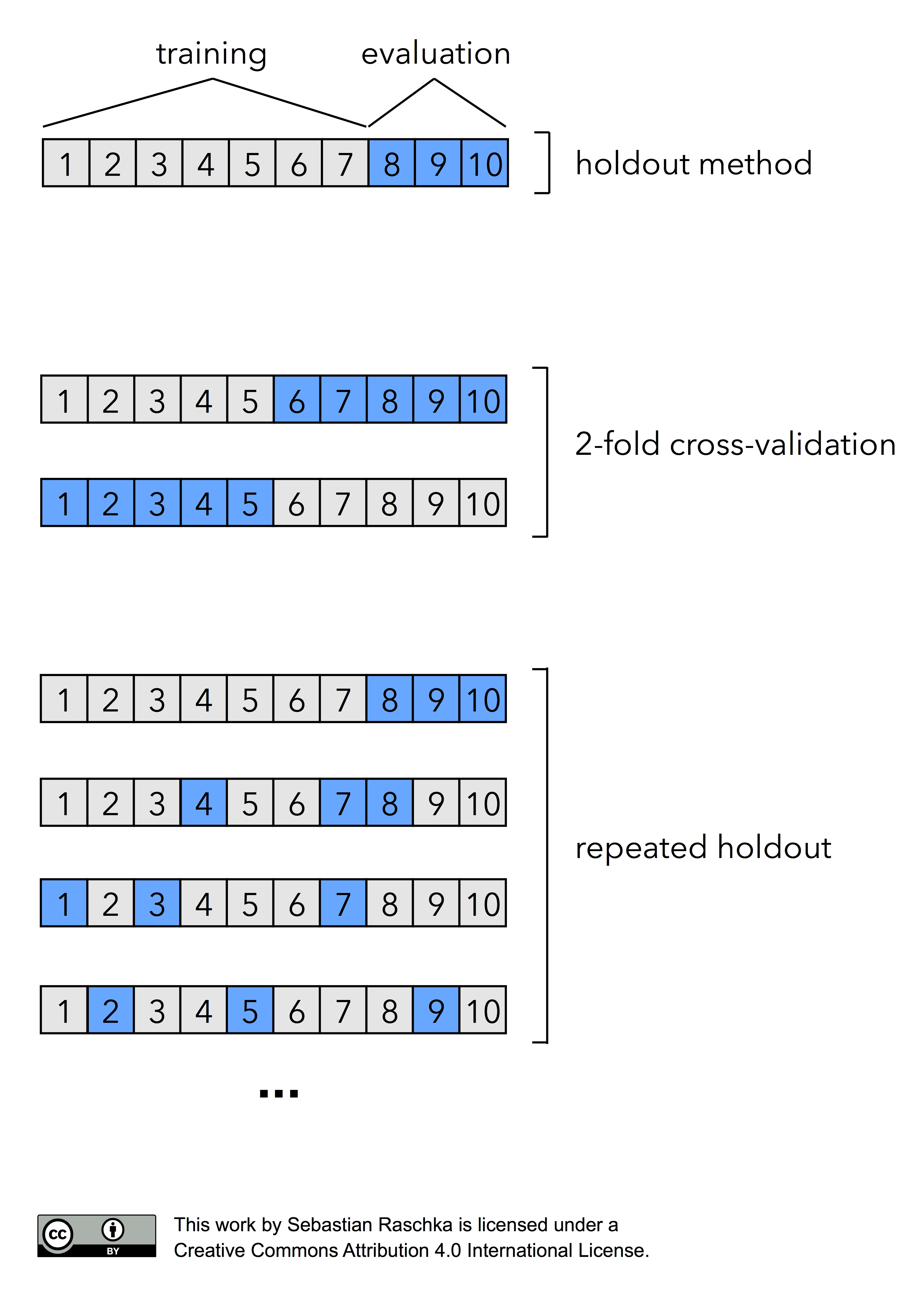
At this point, you may wonder why we chose k=5 to illustrate k-fold cross-validation in the previous section. One reason is that it makes it easier to illustrate k-fold cross-validation compactly. Moreover, k=5 is also a common choice in practice, since it is computationally less expensive compared to larger values of k. If k is too small, though, we may increase the pessimistic bias of our estimate (since less training data is available for model fitting), and the variance of our estimate may increase as well since the model is more sensitive to how we split the data (later, we will discuss experiments that suggest k=10 as a good choice for k).
In fact, there are two prominent, special cases of k-fold cross validation: k=2 and k=n. Most literature describes 2-fold cross-validation as being equal to the holdout method. However, this statement would only be true if we perform the holdout method by rotating the training and validation set in two rounds (i.e., using exactly 50% data for training and 50% of the samples for validation in each round, swapping these sets, repeating the training and evaluation procedure, and eventually computing the performance estimate as the arithmetic mean of the two performance estimates on the validation sets). Given how the holdout method is most commonly used though, I like to describe the holdout method and 2-fold cross-validation as two different processes as illustrated in the figure below:
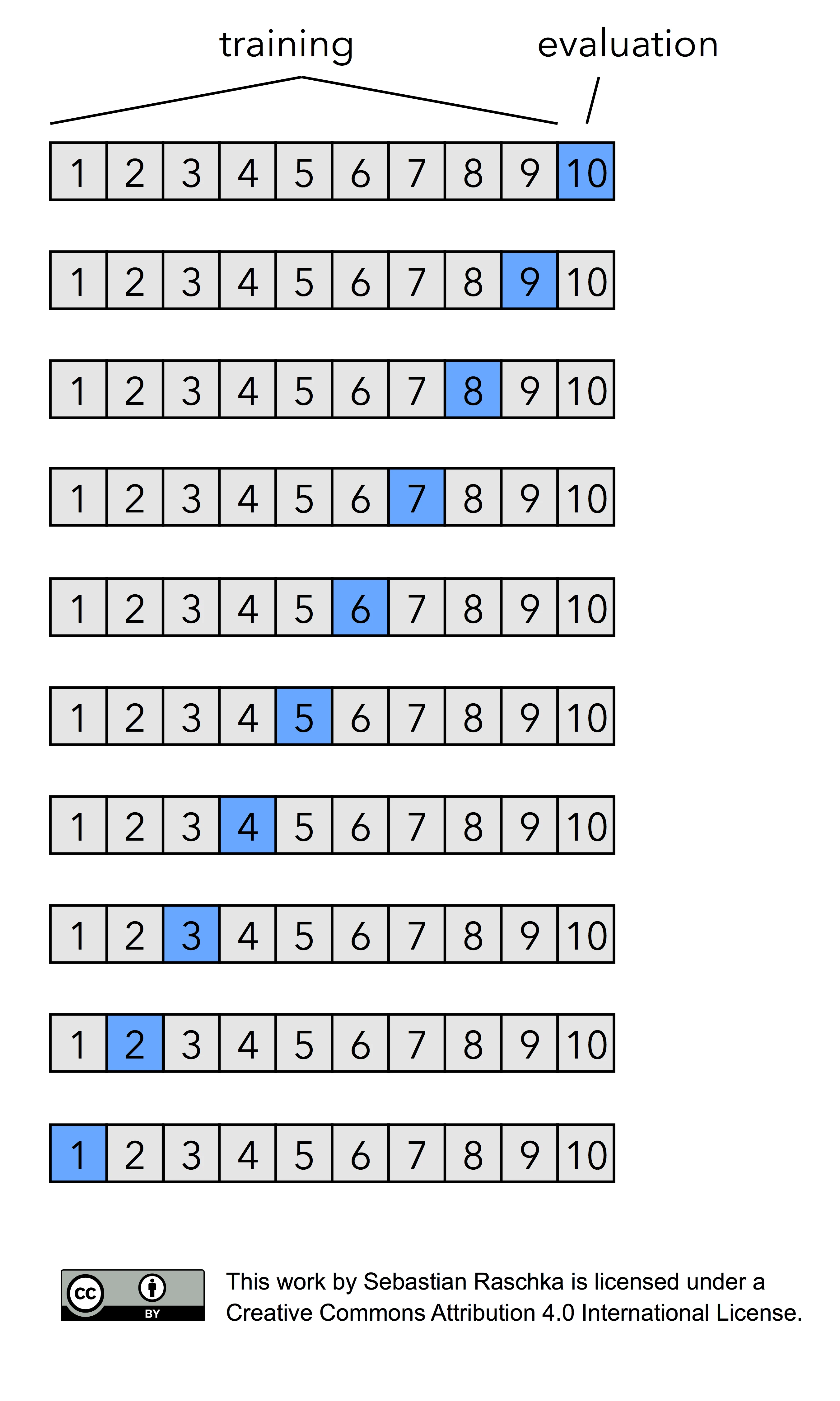
Now, if we set k=n, that is, if set the number of folds as being equal to the number of training instances, we refer to the k-fold cross-validation process as Leave-one-out cross-validation (LOOCV). In each iteration during LOOCV, we fit a model to n-1 samples of the dataset and evaluate it on the single, remaining data point. Although this process is computationally expensive, given that we have n iterations, it can be useful for small datasets, cases where withholding data from the training set would be too wasteful.
Several studies compared different values of k in k-fold cross-validation, analyzing how the choice of k affects the variance and the bias of the estimate. Unfortunately, there is no Free Lunch though as shown by Yohsua Bengio and Yves Grandvalet in “No unbiased estimator of the variance of k-fold cross-validation.”
The main theorem shows that there exists no universal (valid under all distributions) unbiased estimator of the variance of K-fold cross-validation. (Bengio and Grandvalet, 2004)
However, we may still be interested in finding a “sweet spot,” a value that seems to be a good trade-off between variance and bias in most cases, and we will continue the bias-variance trade-off discussion in the next section. For now, let’s conclude this section by looking at an interesting research project where Hawkins and others compared performance estimates via LOOCV to the holdout method and recommend the LOOCV over the latter — if computationally feasible.
[…] where available sample sizes are modest, holding back compounds for model testing is ill-advised. This fragmentation of the sample harms the calibration and does not give a trustworthy assessment of fit anyway. It is better to use all data for the calibration step and check the fit by cross-validation, making sure that the cross-validation is carried out correctly. […] The only motivation to rely on the holdout sample rather than cross-validation would be if there was reason to think the cross-validation not trustworthy — biased or highly variable. But neither theoretical results nor the empiric results sketched here give any reason to disbelieve the cross-validation results. (Hawkins and others, 2003)
These conclusions are partly based on the experiments carried out in this study using a 469-sample dataset. The following table summarizes the finding in a comparison of different Ridge Regression models:
| experiment | mean | standard deviation |
|---|---|---|
| true R2—q2 | 0.010 | 0.149 |
| true R2—hold 50 | 0.028 | 0.184 |
| true R2—hold 20 | 0.055 | 0.305 |
| true R2—hold 10 | 0.123 | 0.504 |
In rows 1-4, Hawkins and others used 100-sample training sets to compare different methods of model evaluation. The first row corresponds to an experiment where the researchers used LOOCV and fit regression models to 100-sample training subsets. The reported “mean” refers to the averaged difference between the true coefficiants of determination and the coefficients of determination obtained via LOOCV (here called q2) after repeating this procedure on different 100-sample training sets. In rows 2-4, the researchers used the holdout method for fitting models to 100-sample training sets, and they evaluated the performances on holdout sets of sizes 10, 20, and 50 samples. Each experiment was repeated 75 times, and the mean column shows the average difference between the estimated R2 and true R2 values. As we can see, the estimate obtained via LOOCV (q2) is closest to the true R2. The estimates obtained from the 50-test sample holdout method are also passable, though. Based on these particular experiments, I agree with the researchers’ conclusion:
Taking the third of these points, if you have 150 or more compounds available, then you can certainly make a random split into 100 for calibration and 50 or more for testing. However it is hard to see why you would want to do this.
One reason why we may prefer the holdout method may be concerns about computational efficiency, if our dataset is sufficiently large. As a rule of thumb, we can say that the pessimistic bias and large variance concerns are less problematic the larger the dataset. Moreover, it is not uncommon to repeat the k-fold cross-validation procedure with different random seeds in hope to obtain a “more robust” estimate. For instance, if we repeated a 5-fold cross-validation run 100 times, we would compute the performance estimate for 500 test folds report the cross-validation performance as the arithmetic mean of these 500 folds. (Although this is commonly done in practice, we note that the test folds are now overlapping.) However, there’s no point in repeating LOOCV, since LOOCV always produces the same splits.
K and the Bias-variance Trade-off
Based on the experimental evidence that we saw in the previous section, we may prefer LOOCV over single train/test splits via the holdout method for small and moderately sized datasets. In addition, we can think of the LOOCV estimate as being approximately unbiased: the pessimistic bias of LOOCV (k=n) is intuitively lower compared k<n-fold cross-validation, since almost all (for instance, n-1) training samples are available for model fitting.
While LOOCV is almost unbiased, one downside of using LOOCV over k-fold cross-validation with k<n is the large variance of the LOOCV estimate. First, we have to note that LOOCV is defect when using a discontinuous loss-function such as the 0-1 loss in classification or even in continuous loss functions such as the mean-squared-error. Often, it is said that LOOCV
… [LOOCV has] high variance because the test set only contains one sample. (Tan and others, 2005)
… [LOOCV] is highly variable, since it is based upon a single observation (x1, y1). (Gareth and others, 2013)
These statements are certainly true if we refer to the variance between folds. Remember that if we use the 0-1 loss function (the prediction is either correct or not), we could consider each prediction as a Bernoulli trial, and the number of correct predictions \(X\) is following a binomial distribution \(X \sim B(n, p)\), where \(n \in \mathbb{N} \text{ and } p \in [0,1]\); the variance of a binomial distribution is defined as \(\sigma^2 = np(1-p)\).
We can estimate the variability of a statistic (here: the performance of the model) from the variability of that statistic between subsamples. Obviously though, the variance between folds is a poor estimate of the variance of the LOOCV estimate — the variability due to randomness in our training data. Now, when we are talking about the variance of LOOCV, we typically mean the difference in the results that we would get if we repeated the resampling procedure multiple times on different data samples from the underlying distribution. Thus, a more interesting point has been made by Hastie, Tibshirani, and Friedman:
With K = N, the cross-validation estimator is approximately unbiased for the true (expected) prediction error, but can have high variance because the N “training sets” are so similar to one another. (Hastie and others, 2009)
Or in other words, we can attribute the high variance to the well-known fact that the mean of highly correlated variables has a higher variance than the mean of variables that are not highly correlated. Maybe, this can intuitively be explained by looking at the relationship between covariance (\(\text{cov}\)) and variance (\(\sigma^2\)):
\[\text{cov}_{X, X} = \sigma^2_{X}\]Proof: \(\text{Let } \mu = E(X), { then } \quad \text{cov}_{X, X} = E\left[(X - \mu)^2\right] = \sigma^{2}_{X}\)
And the relationship between covariance \(\text{cov}_{X, Y}\) and correlation \(\rho_{X, Y}\) (X and Y are random variables) is defined as
\[\text{cov}_{X, Y} = \rho_{X, Y} \; \sigma_X \sigma_Y,\]where
\[\text{cov}_{X, Y} = E [(X - \mu_X)(Y - \mu_Y)]\]and
\[\rho_{X, Y} = E [(X - \mu_X)(Y - \mu_Y)] / (\sigma_X \sigma_Y).\]The large variance that is often associated with LOOCV has also been observed in empirical studies — for example, I really recommend reading the excellent paper A Study of Cross-Validation and Bootstrap for Accuracy Estimation and Model Selection (Kohavi, 1995) by Ron Kohavi.
Now that we established that LOOCV estimates are generally associated with a large variance and a small bias, how does this method compare to k-fold cross-validation with other choices for k and the bootstrap method? In Part II, we mentioned the pessimistic bias of the standard bootstrap method, where the training set asymptotically (only) contains 0.632 of the samples from the original dataset; 2- or 3-fold cross-validation has about the same problem. We discussed the 0.632 Bootstrap that was designed to address this pessimistic bias issue. However, Kohavi also observed in his experiments (Kohavi, 1995) that the bias in bootstrap was still extremely large for certain real-world datasets (now, optimistically biased) compared to k-fold cross-validation. Eventually, Kohavi’s experiments on various real-world datasets suggest that 10-fold cross-validation offers the best trade-off between bias and variance. Furthermore, other researchers found that repeating k-fold cross-validation can increase the precision of the estimates while still maintaining a small bias (Molinaro and others, 2005; Kim, 2009).
Before moving on to model selection, let’s summarize this discussion of the bias-variance trade-off by listing the general trends when increasing the number of folds or k:
- the bias of the performance estimator decreases (more accurate)
- the variance of the performance estimators increases (more variability)
- computational cost increases (more iterations, larger training sets during fitting)
- exception: decreasing the value of k in k-fold cross-validation to small values (e.g., 2 or 3) also increases the variance on small datasets due to random sampling effects.
Model Selection via K-fold Cross-validation
Previously, we used k-fold cross-validation for model evaluation. Now, we are going to take things further and use the k-fold cross-validation method for model selection. Again, the key idea is to keep an independent test dataset, that we withhold from during training and model selection, to avoid the leaking of test data in the training stage:
Although, the figure above might seem somewhat complicated at first glance, the process is quite simple and similar to the “three-way holdout” workflow that we discussed at the beginning of this article. Let’s walk through it step by step.

Similar to the holdout method, we split our dataset into two parts, a training and an independent test set; we tuck away the test set for the final model evaluation step at the end.
In the second step, we can now experiment with various hyperparameter settings; we could use Bayesian Optimization, Randomized Search, or plain old Grid Search. For each hyperparameter configuration, we apply the k-fold cross-validation on the training set, resulting in multiple models and performance estimates.
Taking the hyperparameter settings that correspond to the best-performing model, we can then use the complete training set for model fitting.

Now it’s time to make use of the independent test set that we withheld; we use this test set to evaluate the model that we obtained from step 3.

Finally, when we completed the evaluation stage, we can fit a model to all our data, which could be the model for (the so-called) deployment.
When we browse the deep learning literature, we often find that that the 3-way holdout method is the method of choice when it comes to model evaluation; it is also common in older (non-deep learning literature) as well. As mentioned earlier, the three-way holdout may be preferred over k-fold cross-validation since the former is computationally cheap in comparison. Aside from computational efficiency concerns, we only use deep learning algorithms when we have relatively large sample sizes anyway, scenarios where we don’t have to worry about high variance — due to sensitivity of our estimates towards how we split the dataset for training, validation, and testing — so much.
The Law of Parsimony
Now that we discussed model selection in the previous section, let us take a moment and consider the Law of Parsimony aka Occam’s Razor:
Among competing hypotheses, the one with the fewest assumptions should be selected.
Or to say it with other words, using one of my favorite quotes:
“Everything should be made as simple as possible, but not simpler.” — Albert Einstein
In model selection practice, we can apply Occam’s razor using the one-standard error method as follows:
- Consider the numerically optimal estimate and its standard error.
- Select the model whose performance is within one standard error of the value obtained in step 1 (Breiman and others, 1984).
Although, we may prefer simpler models for several reasons, Pedro Domingos made a good point regarding the performance of “complex” models. Here’s an excerpt from his recent article, “Ten Myths About Machine Learning:”
Simpler models are more accurate. This belief is sometimes equated with Occam’s razor, but the razor only says that simpler explanations are preferable, not why. They’re preferable because they’re easier to understand, remember, and reason with. Sometimes the simplest hypothesis consistent with the data is less accurate for prediction than a more complicated one. Some of the most powerful learning algorithms output models that seem gratuitously elaborate — sometimes even continuing to add to them after they’ve perfectly fit the data — but that’s how they beat the less powerful ones.
Again, there are several reasons why we may prefer a simpler model if its performance is within a certain, acceptable range — for example, using the one-standard error method. Although a simpler model may not be the most “accurate” one, it may be computationally more efficient, easier to implement, and easier to understand and reason with compared to more complicated alternatives.
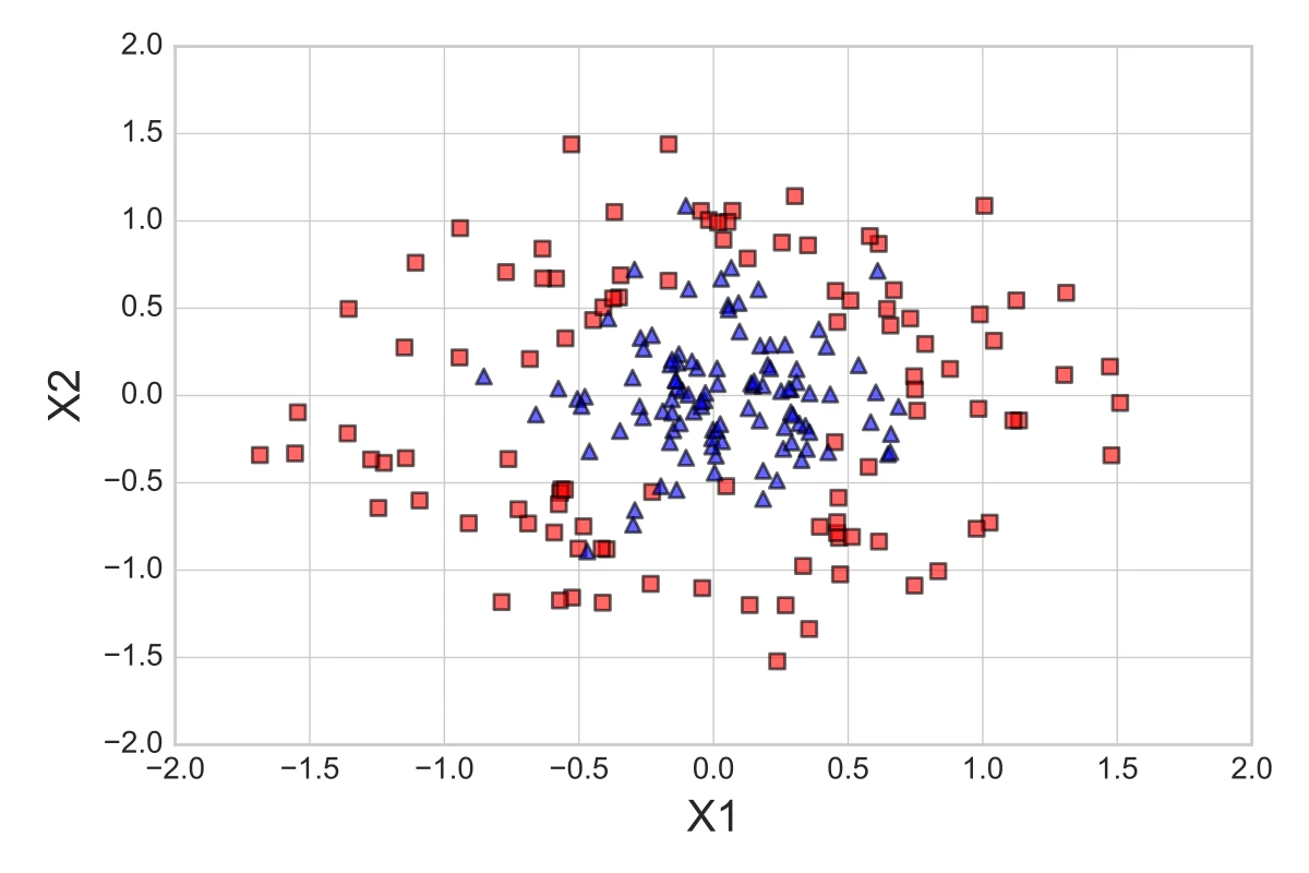
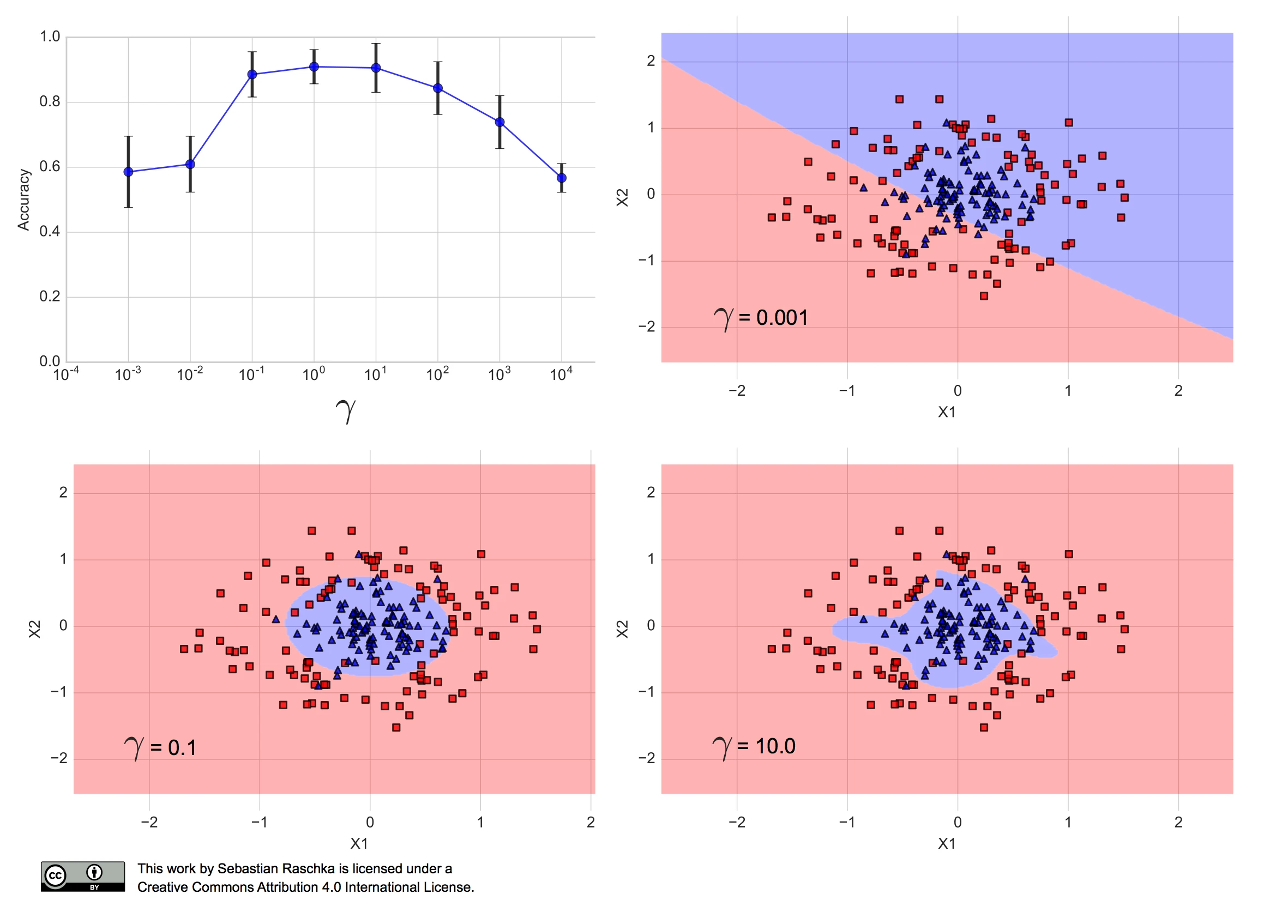
To see how the one-standard error method works in practice, let us apply it to a simple toy dataset: 300 datapoints, concentric circles, and a uniform class distribution (150 samples from class 1 and 150 samples from class 2). First, we split the dataset into two parts, 70% training data and 30% test data, using stratification to maintain equal class proportions. The 210 samples from the training dataset are shown below:
Say we want to optimize the Gamma hyperparameter of a Support Vector Machine (SVM) with a non-linear Radial Basis Function-kernel (RBF-kernel), where \(\gamma\) is the free parameter of the Gaussian RBF:
\[K(x_i, x_j) = exp(-\gamma || x_i - x_j ||^2), \gamma > 0\](Intuitively, we can think of the Gamma as a parameter that controls the influence of single training samples on the decision boundary.)
When I ran the RBF-kernel SVM algorithm with different Gamma values over the training set, using stratified 10-fold cross-validation, I obtained the following performance estimates, where the error bars are the standard errors of the cross-validation estimates:
(The code for producing the plots shown in this article can be found in this Jupyter Notebook on GitHub.)
We can see that Gamma values between 0.1 and 100 resulted in a prediction accuracy of 80% or more. Furthermore, we can see that \(\gamma=10.0\) results in a fairly complex decision boundary, and \(\gamma=0.001\) results in a decision boundary that is too simple to separate the two classes. In fact, \(\gamma=0.1\) seems like a good trade-off between the two aforementioned models — the performance of the corresponding model falls within one standard error of the best performing model with \(\gamma=0\) or \(\gamma=10\).
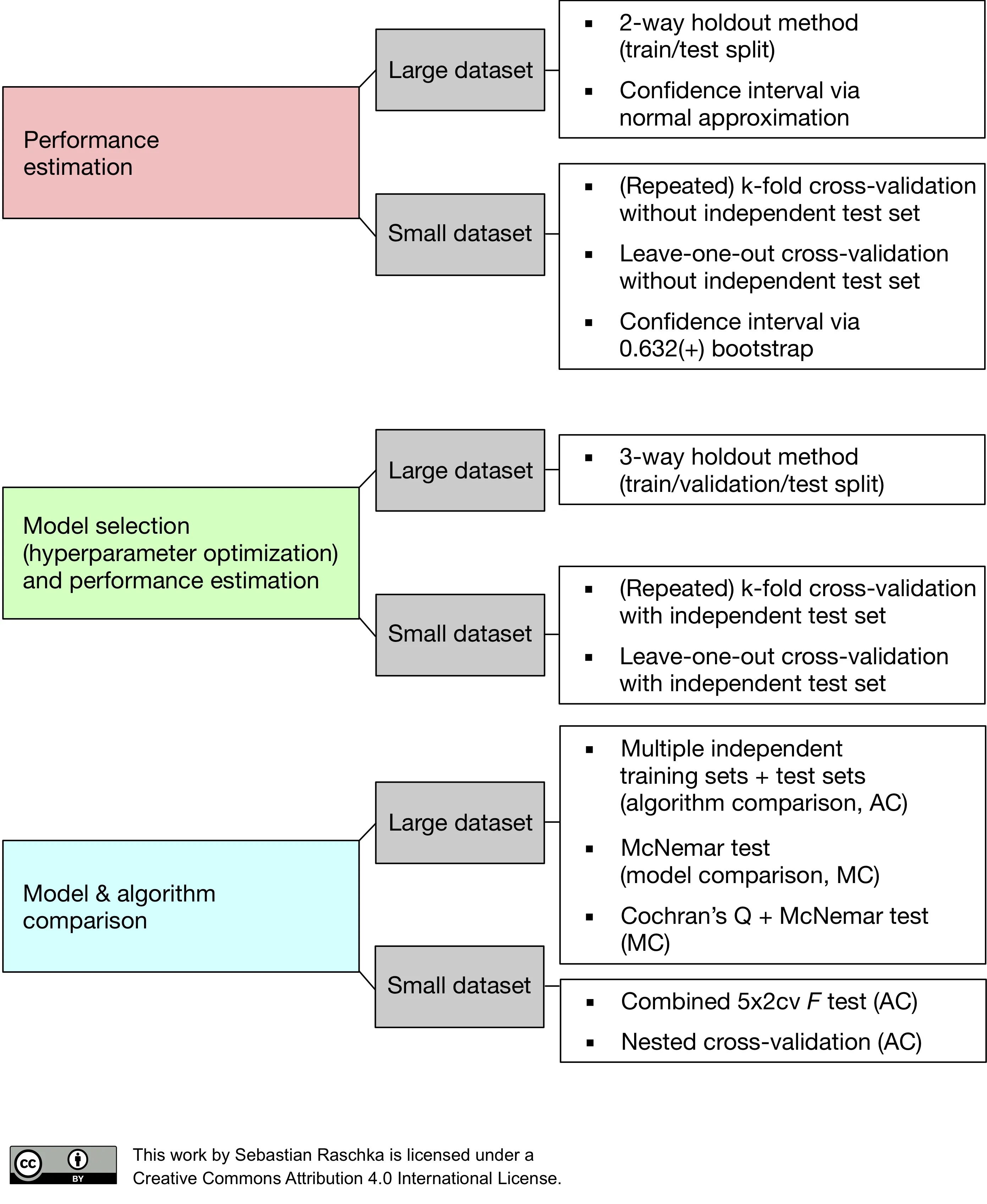
Summary and conclusion
There are many ways for evaluating the generalization performance of predictive models. So far, we have seen the holdout method, different flavors of the bootstrap approach, and k-fold cross-validation. In my opinion, the holdout method is absolutely fine for model evaluation when working with relatively large sample sizes. If we are into hyperparameter tuning, we may prefer 10-fold cross-validation, and Leave-One-Out cross-validation is a good option if we are working with small sample sizes. When it comes to model selection, again, the “three-way” holdout method may be a good choice due to computational limitations; a good alternative is k-fold cross-validation with an independent test set. An even better method for model selection or algorithm selection is nested cross-validation, a method that we will discuss in Part IV.
Thank you for reading. If you liked this content, you can also find me on Twitter, where I share more helpful content.
What’s Next
In the next part of this series, we will discuss hypothesis tests and methods for algorithm selection in more detail.
Say we want to hire a stock market analyst. To find a good stock market analyst, let’s assume we asked our candidates to predict whether certain stock prices go up or down in the next 10 days, prior to the interview. A good candidate should get at least 8 out of these 10 predictions correct. Without having any knowledge about how stocks work, I would say that our probability of correctly predicting the trend each day is 50% — that’s a coin-flip each day. So, if we just interviewed one coin-flipping candidate, her chance of being right 8 out of 10 times would be 0.0547:
\[\frac{ {10 \choose 8} + {10 \choose 9} + {10 \choose 10}}{2^{10} } = 0.0547.\]In other words, we can say that this candidate’s predictive performance is unlikely due to chance. However, say we didn’t just invite one single interviewee: we invited 100. If we’d asked these 100 interviewers for their predictions. Assuming that no candidate has a clue about how stocks work, and everyone was guessing randomly, the probability that at least one of the candidates got 8 out of 10 predictions correct is:
\[1 - (1 - 0.0547)^{100} = 0.9964.\]So, shall we assume that a candidate who got 8 out of 10 predictions correct was not simply guessing randomly? We will continue this discussion on hypothesis tests, comparisons between learning algorithms in Part IV.
References
- Bengio, Yoshua, and Yves Grandvalet. 2004. “No Unbiased Estimator of the Variance of K-Fold Cross-Validation.” J. Mach. Learn. Res. 5 (December). JMLR.org: 1089–1105.
- Breiman, Leo, Jerome Friedman, Charles J Stone, and Richard A Olshen. 1984. Classification and Regression Trees. CRC press. Breiman, Leo. 1996. “Heuristics of Instability and Stabilization in Model Selection.” The Annals of Statistics 24 (6). Institute of Mathematical Statistics: 2350–83.
- Hastie, Trevor, Robert Tibshirani, and J. H. Friedman. “7.10.1 K-Fold Cross-Validation.” In The Elements of Statistical Learning: Data Mining, Inference, and Prediction. 2nd ed. New York: Springer, 2009.
- Hawkins, Douglas M., Subhash C. Basak, and Denise Mills. 2003. “Assessing Model Fit by Cross-Validation.” Journal of Chemical Information and Computer Sciences 43 (2). American Chemical Society: 579–86.
- Kohavi, Ron. 1995. “A Study of Cross-Validation and Bootstrap for Accuracy Estimation and Model Selection.” International Joint Conference on Artificial Intelligence 14 (12): 1137–43
- James, Gareth, Daniela Witten, Trevor Hastie, and Robert Tibshirani. “5.1 Cross-Validation” In An Introduction to Statistical Learning: With Applications in R. Vol. 6. New York: Springer, 2013.
- Jiang, Wenyu, and Richard Simon. 2007. “A Comparison of Bootstrap Methods and an Adjusted Bootstrap Approach for Estimating the Prediction Error in Microarray Classification.” Statistics in Medicine 26 (29): 5320–34.
- Kim, Ji-Hyun. 2009. “Estimating Classification Error Rate: Repeated Cross-Validation, Repeated Hold-out and Bootstrap.” Computational Statistics & Data Analysis 53 (11): 3735–45.
- Molinaro, Annette M, Richard Simon, and Ruth M Pfeiffer. 2005. “Prediction Error Estimation: A Comparison of Resampling Methods.” Bioinformatics (Oxford, England) 21 (15). Oxford University Press: 3301–7.
- Refaeilzadeh, Payam, Lei Tang, and Huan Liu. 2007. “On Comparison of Feature Selection Algorithms.” In Proceedings of AAAI Workshop on Evaluation Methods for Machine Learning II, 34–39.
- Tan, Pang-Ning, Michael Steinbach, and Vipin Kumar. “4. Classification: Basic Concepts, Decision Trees, and Model Evaluation.” In Introduction to Data Mining. Boston: Pearson Addison Wesley, 2005.
Read Next
 Scientific Computing in Python: Introduction to NumPy and Matplotlib
Beginner's guide to NumPy and Matplotlib for scientific computing: arrays, indexing, broadcasting, linear algebra, and plotting with Python code examples.
Scientific Computing in Python: Introduction to NumPy and Matplotlib
Beginner's guide to NumPy and Matplotlib for scientific computing: arrays, indexing, broadcasting, linear algebra, and plotting with Python code examples.
 Model evaluation, model selection, and algorithm selection in machine learning
Part 4 of the model evaluation series explaining statistical tests, algorithm comparisons, corrected resampled tests, and nested cross-validation.
Model evaluation, model selection, and algorithm selection in machine learning
Part 4 of the model evaluation series explaining statistical tests, algorithm comparisons, corrected resampled tests, and nested cross-validation.
 Generating Gender-Neutral Face Images with Semi-Adversarial Neural Networks to Enhance Privacy
I thought that it would be nice to have short and concise summaries of recent projects handy, to share them with a more general audience, including...
Generating Gender-Neutral Face Images with Semi-Adversarial Neural Networks to Enhance Privacy
I thought that it would be nice to have short and concise summaries of recent projects handy, to share them with a more general audience, including...

If you read the book and have a few minutes to spare, I'd really appreciate a brief review. It helps us authors a lot!
Your support means a great deal! Thank you!