Model evaluation, model selection, and algorithm selection in machine learning

A single-PDF version of Model Evaluation parts 1-4 is available on arXiv: https://arxiv.org/abs/1811.12808

Introduction

Machine learning has become a central part of our life – as consumers, customers, and hopefully as researchers and practitioners! Whether we are applying predictive modeling techniques to our research or business problems, I believe we have one thing in common: We want to make “good” predictions! Fitting a model to our training data is one thing, but how do we know that it generalizes well to unseen data? How do we know that it doesn’t simply memorize the data we fed it and fails to make good predictions on future samples, samples that it hasn’t seen before? And how do we select a good model in the first place? Maybe a different learning algorithm could be better-suited for the problem at hand?

Model evaluation is certainly not just the end point of our machine learning pipeline. Before we handle any data, we want to plan ahead and use techniques that are suited for our purposes. In this article, we will go over a selection of these techniques, and we will see how they fit into the bigger picture, a typical machine learning workflow.

Performance Estimation: Generalization Performance Vs. Model Selection

Let’s start this section with a simple Q&A:

Q: “How do we estimate the performance of a machine learning model?”

A: “First, we feed the training data to our learning algorithm to learn a model. Second, we predict the labels of our test set. Third, we count the number of wrong predictions on the test dataset to compute the model’s prediction accuracy.”

Not so fast! Depending on our goal, estimating the performance of a model is not that trivial, unfortunately. Maybe we should address the previous question from another angle: “Why do we care about performance estimates at all?” Ideally, the estimated performance of a model tells how well it performs on unseen data – making predictions on future data is often the main problem we want to solve in applications of machine learning or the development of novel algorithms. Typically, machine learning involves a lot of experimentation, though — for example, the tuning of the internal knobs of a learning algorithm, the so-called hyperparameters. Running a learning algorithm over a training dataset with different hyperparameter settings will result in different models. Since we are typically interested in selecting the best-performing model from this set, we need to find a way to estimate their respective performances in order to rank them against each other. Going one step beyond mere algorithm fine-tuning, we are usually not only experimenting with the one single algorithm that we think would be the “best solution” under the given circumstances. More often than not, we want to compare different algorithms to each other, oftentimes in terms of predictive and computational performance.

Let us summarize the main points why we evaluate the predictive performance of a model:

1. We want to estimate the generalization performance, the predictive performance of our model on future (unseen) data.
2. We want to increase the predictive performance by tweaking the learning algorithm and selecting the best performing model from a given hypothesis space.
3. We want to identify the machine learning algorithm that is best-suited for the problem at hand; thus, we want to compare different algorithms, selecting the best-performing one as well as the best performing model from the algorithm’s hypothesis space.

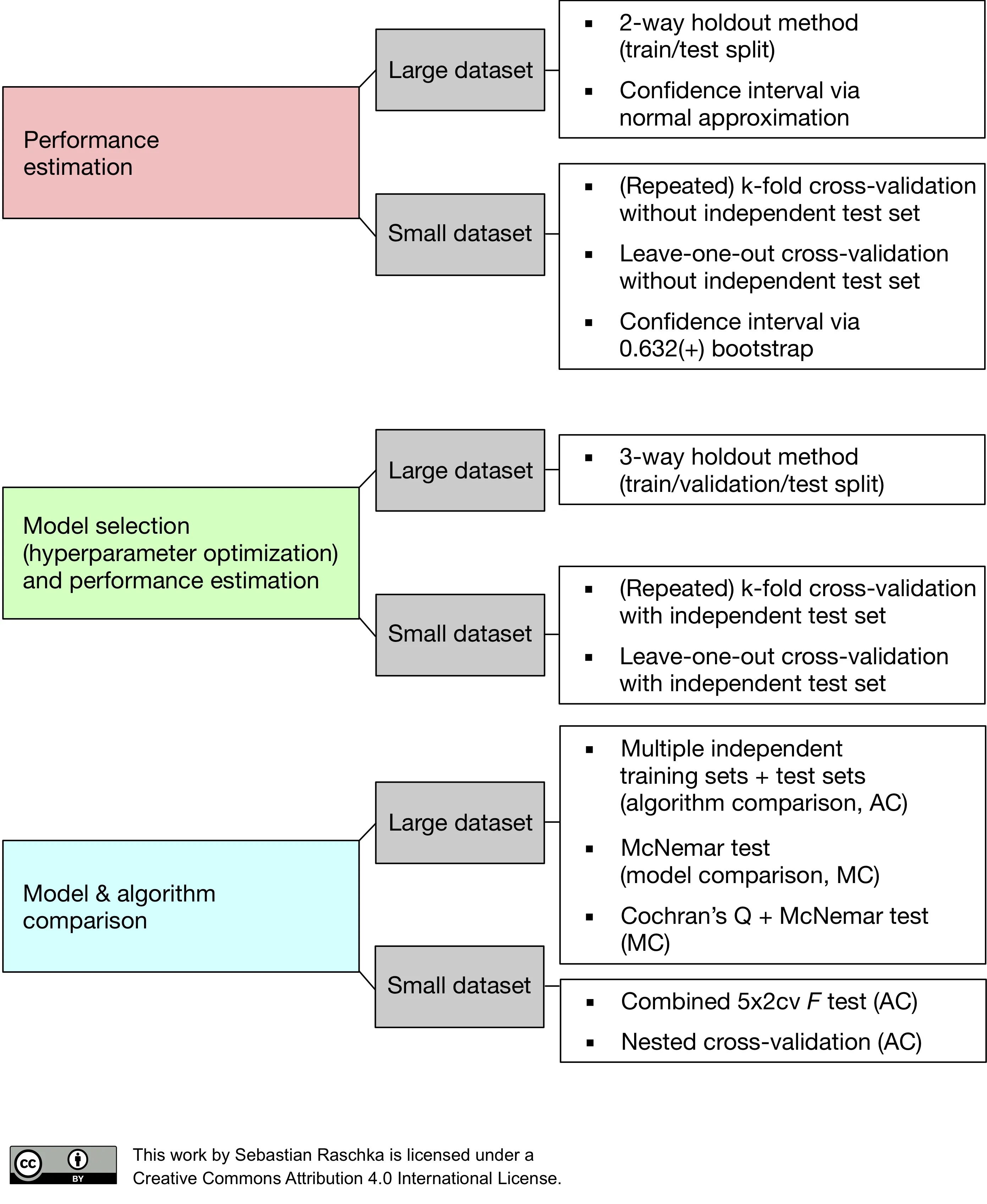
Although these three sub-tasks listed above have all in common that we want to estimate the performance of a model, they all require different approaches. We will discuss some of the different methods for tackling these sub-tasks in this article.

Of course, we want to estimate the future performance of a model as accurately as possible. However, if there’s one key take-away message from this article, it is that biased performance estimates are perfectly okay in model selection and algorithm selection if the bias affects all models equally. If we rank different models or algorithms against each other in order to select the best-performing one, we only need to know the “relative” performance. For example, if all our performance estimates are pessimistically biased, and we underestimate their performances by 10%, it wouldn’t affect the ranking order. More concretely, if we have three models with prediction accuracy estimates such as

M2: 75% > M1: 70% > M3: 65%,

we would still rank them the same way if we add a 10% pessimistic bias:

M2: 65% > M1: 60% > M3: 55%.

On the contrary, if we report the future prediction accuracy of the best ranked model (M2) to be 65%, this would obviously be quite inaccurate. Estimating the absolute performance of a model is probably one of the most challenging tasks in machine learning.

Assumptions and Terminology

Model evaluation is certainly a complex topic. To make sure that we don’t diverge too much from the core message, let us make certain assumptions and go over some of the technical terms that we will use throughout this article.

i.i.d.

We assume that our samples are i.i.d (independent and identically distributed), which means that all samples have been drawn from the same probability distribution and are statistically independent from each other. A scenario where samples are not independent would be working with temporal data or time-series data.

Supervised learning and classification

This article will focus on supervised learning, a subcategory of machine learning where our target values are known in our available dataset. Although many concepts also apply to regression analysis, we will focus on classification, the assignment of categorical target labels to the samples.

0-1 loss and prediction accuracy

In the following article, we will focus on the prediction accuracy, which is defined as the number of all correct predictions divided by the number of samples. We compute the prediction accuracy as the number of correct predictions divided by the number of samples n. Or in more formal terms, we define the prediction accuracy ACC as

where the prediction error ERR is computed as the expected value of the 0-1 loss over n samples in a dataset S:

The 0-1 loss \(L(\cdot)\) is defined as

where \(y_i\) is the ith true class label and \(\hat{y_i}\) the ith predicted class label, respectively.

Our objective is to learn a model h that has a good generalization performance. Such a model maximizes the prediction accuracy or, vice versa, minimizes the probability, C(h), of making a wrong prediction

where \(D\) is the generating distribution our data has been drawn from, \(\mathbf{x}\) is the feature vector of a sample with class label \(y\).

Lastly, since we will mostly refer to the prediction accuracy (instead of the error) throughout this series of articles, we will use Dirac’s Delta function

so that

\(\delta\big( L(\hat{y_i}, y_i)\big) = 1\) if \(\hat{y_i} = y_i\)

and

\(\delta\big( L(\hat{y_i}, y_i)\big) = 0\) if \(\hat{y_i} \neq y_i.\)

(Please note that we use “accuracy” as a performance metric to keep the discussion general and simple, without digressing into a discussion about different performance metrics. Depending on your application, you may want to consider different performance metrics.)

Bias

When we use the term bias in this article, we refer to the statistical bias (in contrast to the bias in a machine learning system). In general terms, the bias of an estimator \(\hat{\beta}\) is the difference between its expected value \(E[\hat{\beta}]\) and the true value of a parameter \(\beta\) being estimated.

So, if \(E\big[\hat{\beta}\big] - \beta = 0\), then \(\hat{\beta}\) is an unbiased estimator of \(\beta\). More concretely, we compute the prediction bias as the difference between the expected prediction accuracy of our model and the true prediction accuracy. For example, if we compute the prediction accuracy on the training set, this would be an optimistically biased estimate of the absolute accuracy of our model since it would overestimate the true accuracy.

Variance

The variance is simply the statistical variance of the estimator \(\hat{\beta}\) and its expected value \(E[\hat{\beta}]\)

The variance is a measure of the variability of our model’s predictions if we repeat the learning process multiple times with small fluctuations in the training set. The more sensitive the model-building process is towards these fluctuations, the higher the variance.

Finally, let us disambiguate the terms model, hypothesis, classifier, learning algorithms, and parameters:

• Target function: In predictive modeling, we are typically interested in modeling a particular process; we want to learn or approximate a specific, unknown function. The target function \(f(x) = y\) is the true function \(f(\cdot)\) that we want to model.

• Hypothesis: A hypothesis is a certain function that we believe (or hope) is similar to the true function, the target function that we want to model. In context of spam classification, it would be a classification rule we came up with that allows us to separate spam from non-spam emails.

• Model: In the machine learning field, the terms hypothesis and model are often used interchangeably. In other sciences, they can have different meanings: A hypothesis could be the “educated guess” by the scientist, and the model would be the manifestation of this guess to test this hypothesis.

• Learning algorithm: Again, our goal is to find or approximate the target function, and the learning algorithm is a set of instructions that tries to model the target function using our training dataset. A learning algorithm comes with a hypothesis space, the set of possible hypotheses it explores to model the unknown target function by formulating the final hypothesis.

• Classifier: A classifier is a special case of a hypothesis (nowadays, often learned by a machine learning algorithm). A classifier is a hypothesis or discrete-valued function that is used to assign (categorical) class labels to particular data points. In an email classification example, this classifier could be a hypothesis for labeling emails as spam or non-spam. Yet, a hypothesis must not necessarily be synonymous to the term classifier. In a different application, our hypothesis could be a function for mapping study time and educational backgrounds of students to their future, continuous-valued, SAT scores – a continuous target variable, suited for regression analysis.

• Hyperparameters: Hyperparameters are the tuning parameters of a machine learning algorithm — for example, the regularization strength of an L2 penalty in the mean squared error cost function of linear regression, or a value for setting the maximum depth of a decision tree. In contrast, model parameters are the parameters that a learning algorithm fits to the training data – the parameters of the model itself. For example, the weight coefficients (or slope) of a linear regression line and its bias (or y-axis intercept) term are model parameters.

Resubstitution Validation and the Holdout Method

The holdout method is inarguably the simplest model evaluation technique. We take our labeled dataset and split it into two parts: A training set and a test set. Then, we fit a model to the training data and predict the labels of the test set. And the fraction of correct predictions constitutes our estimate of the prediction accuracy — we withhold the known test labels during prediction, of course. We really don’t want to train and evaluate our model on the same training dataset (this is called resubstitution evaluation), since it would introduce a very optimistic bias due to overfitting. In other words, we can’t tell whether the model simply memorized the training data or not, or whether it generalizes well to new, unseen data. (On a side note, we can estimate this so called optimism bias as the difference between the training accuracy and the test accuracy.)

Typically, the splitting of a dataset into training and test sets is a simple process of random subsampling. We assume that all our data has been drawn from the same probability distribution (with respect to each class). And we randomly choose ~2/3 of these samples for our training set and ~1/3 of the samples for our test set. Notice the two problems here?

Stratification

We have to keep in mind that our dataset represents a random sample drawn from a probability distribution; and we typically assume that this sample is representative of the true population – more or less. Now, further subsampling without replacement alters the statistic (mean, proportion, and variance) of the sample. The degree to which subsampling without replacement affects the statistic of a sample is inversely proportional to the size of the sample. Let’s have a look at an example using the Iris dataset, which we randomly divide into 2/3 training data and 1/3 test data:

(The source code can be found here.)

When we randomly divide the dataset into training and test sets, we violate the assumption of statistical independence. The Iris dataset consists of 50 Setosa, 50 Versicolor, and 50 Virginica flowers; the flower species are distributed uniformly:

• 33.3% Setosa
• 33.3% Versicolor
• 33.3% Virginia

If our random function assigns 2/3 of the flowers (100) to the training set and 1/3 of the flowers (50) to the test set, it may yield the following:

• training set → 38 x Setosa, 28 x Versicolor, 34 x Virginica
• test set → 12 x Setosa, 22 x Versicolor, 16 x Virginica

Assuming that the Iris dataset is representative of the true population (for instance, assuming that flowers are distributed uniformly in nature), we just created two imbalanced datasets with non-uniform class distributions. The class ratio that the learning algorithm uses to learn the model is “38.0% / 28.0% / 34.0%”. Then, we evaluate a model on a dataset with a class ratio that is imbalanced in the “opposite” direction: “24.0% / 44.0% / 32.0%”. Unless our learning algorithm is completely insensitive to these small perturbations, this is certainly not ideal. The problem becomes even worse if our dataset has a high class imbalance upfront. In the worst-case scenario, the test set may not contain any instance of a minority class at all. Thus, the common practice is to divide the dataset in a stratified fashion. Stratification simply means that we randomly split the dataset so that each class is correctly represented in the resulting subsets — the training and the test set.

Random subsampling in non-stratified fashion is usually not a big concern if we are working with relatively large and balanced datasets. However, in my opinion, stratified resampling is usually (only) beneficial in machine learning applications. Moreover, stratified sampling is incredibly easy to implement, and Ron Kohavi provides empirical evidence (Kohavi 1995) that stratification has a positive effect on the variance and bias of the estimate in k-fold cross-validation, a technique we will discuss later in this article.

Holdout

Before we dive deeper into the pros and cons of the holdout validation method, let’s take a look at a visual summary of the whole process:

① In the first step, we randomly divide our available data into two subsets: a training and a test set. Setting test data aside is our work-around for dealing with the imperfections of a non-ideal world, such as limited data and resources, and the inability to collect more data from the generating distribution. Here, the test set shall represent new, unseen data to our learning algorithm; it’s important that we only touch the test set once to make sure we don’t introduce any bias when we estimate the generalization accuracy. Typically, we assign 2/3 to the training set, and 1/3 of the data to the test set. Other common training/test splits are 60/40, 70/30, 80/20, or even 90/10.

② After we set our test samples aside, we pick a learning algorithm that we think could be appropriate for the given problem. Now, what about the Hyperparameter Values depicted in the figure above? As a quick reminder, hyperparameters are the parameters of our learning algorithm, or meta-parameters if you will. And we have to specify these hyperparameter values manually – the learning algorithm doesn’t learn them from the training data in contrast to the actual model parameters.

Since hyperparameters are not learned during model fitting, we need some sort of “extra procedure” or “external loop” to optimize them separately – this holdout approach is ill-suited for the task. So, for now, we have to go with some fixed hyperparameter values – we could use our intuition or the default parameters of an off-the-shelf algorithm if we are using an existing machine learning library.

③ Our learning algorithm fit a model in the previous step. The next question is: How “good” is the model that it came up with? That’s where our test set comes into play. Since our learning algorithm hasn’t “seen” this test set before, it should give us a pretty unbiased estimate of its performance on new, unseen data! So, what we do is to take this test set and use the model to predict the class labels. Then, we take the predicted class labels and compare it to the “ground truth,” the correct class labels to estimate its generalization accuracy.

④ Finally, we have an estimate of how well our model performs on unseen data. So, there is no reason for with-holding it from the algorithm any longer.

Since we assume that our samples are i.i.d., there is no reason to assume the model would perform worse after feeding it all the available data. As a rule of thumb, the model will have a better generalization performance if the algorithms uses more informative data – given that it hasn’t reached its capacity, yet.

Pessimistic Bias

Remember that we mentioned two problems when we talked about the test and training split earlier? The first problem was the violation of independence and the changing class proportions upon subsampling. We touched upon the second problem when we walked through the holdout illustration. And in step four, we talked about the capacity of the model, and whether additional data could be useful or not. To follow up on the capacity issue: If our model has NOT reached its capacity, our performance estimate would be pessimistically biased. Assuming that the algorithm could learn a better model from more data, we withheld valuable data that we set aside for estimating the generalization performance (i.e., the test dataset). In the fourth step, we fit a model to the complete dataset, though; however, we can’t estimate its generalization performance, since we’ve now “burned” the test dataset. It’s a dilemma that we cannot really avoid in real-world application, but we should be aware that our estimate of the generalization performance may be pessimistically biased.

Confidence Intervals

Using the holdout method as described above, we computed a point estimate of the generalization accuracy of our model. Certainly, a confidence interval around this estimate would not only be more informative and desirable in certain applications, but our point estimate could be quite sensitive to the particular training/test split (i.e., suffering from high variance).

Another, “simpler,” approach, which is often used in practice (although, I do not recommend it), may be using the familiar equation assuming a Normal Distribution to compute the confidence interval on the mean on a single training-test split under the central limit theorem.

In probability theory, the central limit theorem (CLT) states that, given certain conditions, the arithmetic mean of a sufficiently large number of iterates of independent random variables, each with a well-defined expected value and well-defined variance, will be approximately normally distributed, regardless of the underlying distribution. [Source: https://en.wikipedia.org/wiki/Central_limit_theorem]

This rather naive approach is the so-called “Normal approximation interval. “How does that work? Remember, we compute the prediction accuracy as follows

where \(L(\cdot)\) is a 0-1 loss function and \(n\) is the number of samples in the test set; \(\hat{y}\) is the predicted class label and \(y\) is the actual class label of the ith sample, respectively. So, we could now consider each prediction as a Bernoulli trial, and the number of correct predictions \(X\) is following a binomial distribution \(X \sim B(n, p)\) with \(n\) samples and \(k\) trials, where \(n \in \mathbb{N} \text{ and } p \in [0,1]\):

for \(k = 0, 1, 2, ..., n\), where

(Remember, \(p\) is the probability of success, and \((1-p)\) is the probability of failure – a wrong prediction.)

Now, the expected number of successes is computed as \(\mu = np\), or more concretely, if the estimator has 50% success rate, we expect 20 out of 40 predictions to be correct. The estimate has a variance of \(\sigma^2 = np(1-p) = 10\) and a standard deviation of

Since we are interested in the average number of successes, not its absolute value, we compute the variance of the accuracy estimate as

and the respective standard deviation

Under the normal approximation, we can then compute the confidence interval as

where \(\alpha\) is the error quantile and \(z\) is the \(1 - \frac{alpha}{2}\) quantile of a standard normal distribution. For a typical confidence interval of 95% (alpha=5%), we have z=1.96.

In practice, however, I’d rather recommend repeating the training-test split multiple times to compute the confidence interval on the mean estimate (i.e., averaging the individual runs). In any case, one interesting take-away for now is that having fewer samples in the test set increases the variance (see n in the denominator above) and thus widens the confidence interval.

Thank you for reading. If you liked this content, you can also find me on Twitter, where I share more helpful content.

What’s Next

Since the whole article turned out to be quite lengthy, I decided to split it into multiple parts. In the following parts, we will talk about

• Repeated holdout validation and the bootstrap method for modeling uncertainty in Part II
• The holdout method for hyperparameter tuning — splitting a dataset into three parts: a training, test, and validation set (Part III).
• K-fold cross-validation, a popular alternative to model selection (Part III).
• Nested cross-validation, probably the most common technique for model evaluation with hyperparameter tuning or algorithm selection. (Part IV).

References

• Kohavi, R., 1995. A study of cross-validation and bootstrap for accuracy estimation and model selection. In Ijcai (Vol. 14, No. 2, pp. 1137-1145). [Citation source] [PDF]
• Efron, B. and Tibshirani, R.J., 1994. An introduction to the bootstrap. CRC press. [Citation source] [PDF]