About Feature Scaling and Normalization
– and the effect of standardization for machine learning algorithms
Sections
About standardization
The result of standardization (or Z-score normalization) is that the features will be rescaled so that they’ll have the properties of a standard normal distribution with
\(\mu = 0\) and \(\sigma = 1\)
where \(\mu\) is the mean (average) and \(\sigma\) is the standard deviation from the mean; standard scores (also called z scores) of the samples are calculated as follows:
\[z = \frac{x - \mu}{\sigma}\]Standardizing the features so that they are centered around 0 with a standard deviation of 1 is not only important if we are comparing measurements that have different units, but it is also a general requirement for many machine learning algorithms. Intuitively, we can think of gradient descent as a prominent example (an optimization algorithm often used in logistic regression, SVMs, perceptrons, neural networks etc.); with features being on different scales, certain weights may update faster than others since the feature values \(x_j\) play a role in the weight updates
\[\Delta w_j = - \eta \frac{\partial J}{\partial w_j} = \eta \sum_i (t^{(i)} - o^{(i)})x^{(i)}_{j},\]so that
\(w_j := w_j + \Delta w_j,\) where \(\eta\) is the learning rate, \(t\) the target class label, and \(o\) the actual output. Other intuitive examples include K-Nearest Neighbor algorithms and clustering algorithms that use, for example, Euclidean distance measures – in fact, tree-based classifier are probably the only classifiers where feature scaling doesn’t make a difference.
In fact, the only family of algorithms that I could think of being scale-invariant are tree-based methods. Let’s take the general CART decision tree algorithm. Without going into much depth regarding information gain and impurity measures, we can think of the decision as “is feature x_i >= some_val?” Intuitively, we can see that it really doesn’t matter on which scale this feature is (centimeters, Fahrenheit, a standardized scale – it really doesn’t matter).
Some examples of algorithms where feature scaling matters are:
- k-nearest neighbors with an Euclidean distance measure if want all features to contribute equally
- k-means (see k-nearest neighbors)
- logistic regression, SVMs, perceptrons, neural networks etc. if you are using gradient descent/ascent-based optimization, otherwise some weights will update much faster than others
- linear discriminant analysis, principal component analysis, kernel principal component analysis since you want to find directions of maximizing the variance (under the constraints that those directions/eigenvectors/principal components are orthogonal); you want to have features on the same scale since you’d emphasize variables on “larger measurement scales” more. There are many more cases than I can possibly list here … I always recommend you to think about the algorithm and what it’s doing, and then it typically becomes obvious whether we want to scale your features or not.
In addition, we’d also want to think about whether we want to “standardize” or “normalize” (here: scaling to [0, 1] range) our data. Some algorithms assume that our data is centered at 0. For example, if we initialize the weights of a small multi-layer perceptron with tanh activation units to 0 or small random values centered around zero, we want to update the model weights “equally.” As a rule of thumb I’d say: When in doubt, just standardize the data, it shouldn’t hurt.
About Min-Max scaling
An alternative approach to Z-score normalization (or standardization) is the so-called Min-Max scaling (often also simply called “normalization” - a common cause for ambiguities).
In this approach, the data is scaled to a fixed range - usually 0 to 1.
The cost of having this bounded range - in contrast to standardization - is that we will end up with smaller standard deviations, which can suppress the effect of outliers.
A Min-Max scaling is typically done via the following equation:
\[X_{norm} = \frac{X - X_{min}}{X_{max}-X_{min}}\]Z-score standardization or Min-Max scaling?
“Standardization or Min-Max scaling?” - There is no obvious answer to this question: it really depends on the application.
For example, in clustering analyses, standardization may be especially crucial in order to compare similarities between features based on certain distance measures. Another prominent example is the Principal Component Analysis, where we usually prefer standardization over Min-Max scaling, since we are interested in the components that maximize the variance (depending on the question and if the PCA computes the components via the correlation matrix instead of the covariance matrix; but more about PCA in my previous article).
However, this doesn’t mean that Min-Max scaling is not useful at all! A popular application is image processing, where pixel intensities have to be normalized to fit within a certain range (i.e., 0 to 255 for the RGB color range). Also, typical neural network algorithm require data that on a 0-1 scale.
Standardizing and normalizing - how it can be done using scikit-learn
Of course, we could make use of NumPy’s vectorization capabilities to calculate the z-scores for standardization and to normalize the data using the equations that were mentioned in the previous sections. However, there is an even more convenient approach using the preprocessing module from one of Python’s open-source machine learning library scikit-learn.
For the following examples and discussion, we will have a look at the free “Wine” Dataset that is deposited on the UCI machine learning repository
(http://archive.ics.uci.edu/ml/datasets/Wine).
Forina, M. et al, PARVUS - An Extendible Package for Data Exploration, Classification and Correlation. Institute of Pharmaceutical and Food Analysis and Technologies, Via Brigata Salerno, 16147 Genoa, Italy.
Bache, K. & Lichman, M. (2013). UCI Machine Learning Repository [http://archive.ics.uci.edu/ml]. Irvine, CA: University of California, School of Information and Computer Science.
The Wine dataset consists of 3 different classes where each row correspond to a particular wine sample.
The class labels (1, 2, 3) are listed in the first column, and the columns 2-14 correspond to 13 different attributes (features):
1) Alcohol
2) Malic acid
…
Loading the wine dataset
import pandas as pd
import numpy as np

df = pd.io.parsers.read_csv(
    'https://raw.githubusercontent.com/rasbt/pattern_classification/master/data/wine_data.csv',
     header=None,
     usecols=[0,1,2]
    )

df.columns=['Class label', 'Alcohol', 'Malic acid']

df.head()
| Class label | Alcohol | Malic acid | |
|---|---|---|---|
| 0 | 1 | 14.23 | 1.71 |
| 1 | 1 | 13.20 | 1.78 |
| 2 | 1 | 13.16 | 2.36 |
| 3 | 1 | 14.37 | 1.95 |
| 4 | 1 | 13.24 | 2.59 |
As we can see in the table above, the features Alcohol (percent/volumne) and Malic acid (g/l) are measured on different scales, so that Feature Scaling is necessary important prior to any comparison or combination of these data.
Standardization and Min-Max scaling
from sklearn import preprocessing

std_scale = preprocessing.StandardScaler().fit(df[['Alcohol', 'Malic acid']])
df_std = std_scale.transform(df[['Alcohol', 'Malic acid']])

minmax_scale = preprocessing.MinMaxScaler().fit(df[['Alcohol', 'Malic acid']])
df_minmax = minmax_scale.transform(df[['Alcohol', 'Malic acid']])
print('Mean after standardization:\nAlcohol={:.2f}, Malic acid={:.2f}'
      .format(df_std[:,0].mean(), df_std[:,1].mean()))
print('\nStandard deviation after standardization:\nAlcohol={:.2f}, Malic acid={:.2f}'
      .format(df_std[:,0].std(), df_std[:,1].std()))
Mean after standardization:
Alcohol=0.00, Malic acid=0.00

Standard deviation after standardization:
Alcohol=1.00, Malic acid=1.00
print('Min-value after min-max scaling:\nAlcohol={:.2f}, Malic acid={:.2f}'
      .format(df_minmax[:,0].min(), df_minmax[:,1].min()))
print('\nMax-value after min-max scaling:\nAlcohol={:.2f}, Malic acid={:.2f}'
      .format(df_minmax[:,0].max(), df_minmax[:,1].max()))
Min-value after min-max scaling:
Alcohol=0.00, Malic acid=0.00

Max-value after min-max scaling:
Alcohol=1.00, Malic acid=1.00
Plotting
%matplotlib inline
from matplotlib import pyplot as plt

def plot():
    plt.figure(figsize=(8,6))

    plt.scatter(df['Alcohol'], df['Malic acid'],
            color='green', label='input scale', alpha=0.5)

    plt.scatter(df_std[:,0], df_std[:,1], color='red',
            label='Standardized [$$N  (\mu=0, \; \sigma=1)$$]', alpha=0.3)

    plt.scatter(df_minmax[:,0], df_minmax[:,1],
            color='blue', label='min-max scaled [min=0, max=1]', alpha=0.3)

    plt.title('Alcohol and Malic Acid content of the wine dataset')
    plt.xlabel('Alcohol')
    plt.ylabel('Malic Acid')
    plt.legend(loc='upper left')
    plt.grid()

    plt.tight_layout()

plot()
plt.show()
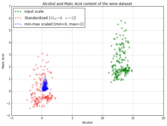
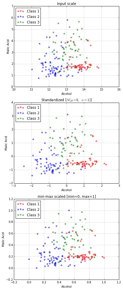
The plot above includes the wine datapoints on all three different scales: the input scale where the alcohol content was measured in volume-percent (green), the standardized features (red), and the normalized features (blue). In the following plot, we will zoom in into the three different axis-scales.
fig, ax = plt.subplots(3, figsize=(6,14))

for a,d,l in zip(range(len(ax)),
               (df[['Alcohol', 'Malic acid']].values, df_std, df_minmax),
               ('Input scale',
                'Standardized [$$N  (\mu=0, \; \sigma=1)$$]',
                'min-max scaled [min=0, max=1]')
                ):
    for i,c in zip(range(1,4), ('red', 'blue', 'green')):
        ax[a].scatter(d[df['Class label'].values == i, 0],
                  d[df['Class label'].values == i, 1],
                  alpha=0.5,
                  color=c,
                  label='Class %s' %i
                  )
    ax[a].set_title(l)
    ax[a].set_xlabel('Alcohol')
    ax[a].set_ylabel('Malic Acid')
    ax[a].legend(loc='upper left')
    ax[a].grid()

plt.tight_layout()

plt.show()
Bottom-up approaches
Of course, we can also code the equations for standardization and 0-1 Min-Max scaling “manually”. However, the scikit-learn methods are still useful if you are working with test and training data sets and want to scale them equally.
E.g.,
std_scale = preprocessing.StandardScaler().fit(X_train)
X_train = std_scale.transform(X_train)
X_test = std_scale.transform(X_test)
Below, we will perform the calculations using “pure” Python code, and an more convenient NumPy solution, which is especially useful if we attempt to transform a whole matrix.
Just to recall the equations that we are using:
Standardization:
\[z = \frac{x - \mu}{\sigma}\]with mean:
\[\mu = \frac{1}{N} \sum_{i=1}^N (x_i)\]and standard deviation:
\[\sigma = \sqrt{\frac{1}{N} \sum_{i=1}^N (x_i - \mu)^2}\]Min-Max scaling:
\[X_{norm} = \frac{X - X_{min}}{X_{max}-X_{min}}\]Vanilla Python
# Standardization

x = [1,4,5,6,6,2,3]
mean = sum(x)/len(x)
std_dev = (1/len(x) * sum([ (x_i - mean)**2 for x_i in x]))**0.5

z_scores = [(x_i - mean)/std_dev for x_i in x]

# Min-Max scaling

minmax = [(x_i - min(x)) / (max(x) - min(x)) for x_i in x]
NumPy
import numpy as np

# Standardization

x_np = np.asarray(x)
z_scores_np = (x_np - x_np.mean()) / x_np.std()

# Min-Max scaling

np_minmax = (x_np - x_np.min()) / (x_np.max() - x_np.min())
Visualization
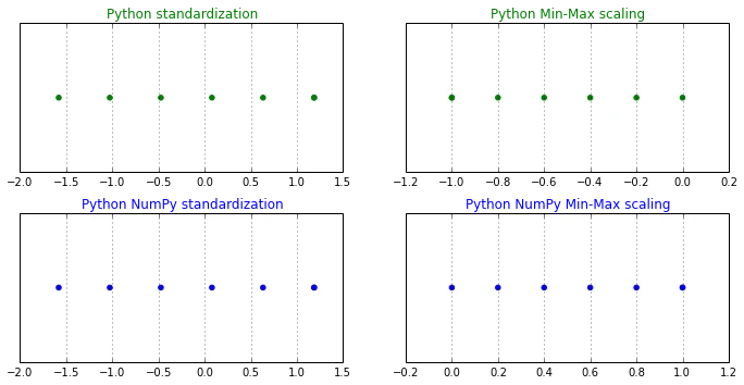
Just to make sure that our code works correctly, let us plot the results via matplotlib.
from matplotlib import pyplot as plt

fig, ((ax1, ax2), (ax3, ax4)) = plt.subplots(nrows=2, ncols=2, figsize=(10,5))

y_pos = [0 for i in range(len(x))]

ax1.scatter(z_scores, y_pos, color='g')
ax1.set_title('Python standardization', color='g')

ax2.scatter(minmax, y_pos, color='g')
ax2.set_title('Python Min-Max scaling', color='g')

ax3.scatter(z_scores_np, y_pos, color='b')
ax3.set_title('Python NumPy standardization', color='b')

ax4.scatter(np_minmax, y_pos, color='b')
ax4.set_title('Python NumPy Min-Max scaling', color='b')

plt.tight_layout()

for ax in (ax1, ax2, ax3, ax4):
    ax.get_yaxis().set_visible(False)
    ax.grid()

plt.show()
The effect of standardization on PCA in a pattern classification task
Earlier, I mentioned the Principal Component Analysis (PCA) as an example where standardization is crucial, since it is “analyzing” the variances of the different features.
Now, let us see how the standardization affects PCA and a following supervised classification on the whole wine dataset.
In the following section, we will go through the following steps:
- Reading in the dataset
- Dividing the dataset into a separate training and test dataset
- Standardization of the features
- Principal Component Analysis (PCA) to reduce the dimensionality
- Training a naive Bayes classifier
- Evaluating the classification accuracy with and without standardization
Reading in the dataset
import pandas as pd

df = pd.io.parsers.read_csv(
    'https://raw.githubusercontent.com/rasbt/pattern_classification/master/data/wine_data.csv',
    header=None,
    )
Dividing the dataset into a separate training and test dataset
In this step, we will randomly divide the wine dataset into a training dataset and a test dataset where the training dataset will contain 70% of the samples and the test dataset will contain 30%, respectively.
from sklearn.cross_validation import train_test_split

X_wine = df.values[:,1:]
y_wine = df.values[:,0]

X_train, X_test, y_train, y_test = train_test_split(X_wine, y_wine,
    test_size=0.30, random_state=12345)
Feature Scaling - Standardization
from sklearn import preprocessing

std_scale = preprocessing.StandardScaler().fit(X_train)
X_train_std = std_scale.transform(X_train)
X_test_std = std_scale.transform(X_test)
Dimensionality reduction via Principal Component Analysis (PCA)
Now, we perform a PCA on the standardized and the non-standardized datasets to transform the dataset onto a 2-dimensional feature subspace.
In a real application, a procedure like cross-validation would be done in order to find out what choice of features would yield a optimal balance between “preserving information” and “overfitting” for different classifiers. However, we will omit this step since we don’t want to train a perfect classifier here, but merely compare the effects of standardization.
from sklearn.decomposition import PCA

# on non-standardized data
pca = PCA(n_components=2).fit(X_train)
X_train = pca.transform(X_train)
X_test = pca.transform(X_test)


# om standardized data
pca_std = PCA(n_components=2).fit(X_train_std)
X_train_std = pca_std.transform(X_train_std)
X_test_std = pca_std.transform(X_test_std)
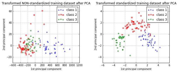
Let us quickly visualize how our new feature subspace looks like (note that class labels are not considered in a PCA - in contrast to a Linear Discriminant Analysis - but I will add them in the plot for clarity).
from matplotlib import pyplot as plt

fig, (ax1, ax2) = plt.subplots(ncols=2, figsize=(10,4))


for l,c,m in zip(range(1,4), ('blue', 'red', 'green'), ('^', 's', 'o')):
    ax1.scatter(X_train[y_train==l, 0], X_train[y_train==l, 1],
        color=c,
        label='class %s' %l,
        alpha=0.5,
        marker=m
        )

for l,c,m in zip(range(1,4), ('blue', 'red', 'green'), ('^', 's', 'o')):
    ax2.scatter(X_train_std[y_train==l, 0], X_train_std[y_train==l, 1],
        color=c,
        label='class %s' %l,
        alpha=0.5,
        marker=m
        )

ax1.set_title('Transformed NON-standardized training dataset after PCA')
ax2.set_title('Transformed standardized training dataset after PCA')

for ax in (ax1, ax2):

    ax.set_xlabel('1st principal component')
    ax.set_ylabel('2nd principal component')
    ax.legend(loc='upper right')
    ax.grid()
plt.tight_layout()

plt.show()
Training a naive Bayes classifier
We will use a naive Bayes classifier for the classification task. If you are not familiar with it, the term “naive” comes from the assumption that all features are “independent”.
All in all, it is a simple but robust classifier based on Bayes’ rule
Bayes’ Rule:
\[P(\omega_j|x) = \frac{p(x|\omega_j) * P(\omega_j)}{p(x)}\]where
-
ω: class label
- \[P(\omega | x): \text{posterior probability}\]
- \[p(x | \omega ): \text{prior probability (or likelihood)}\]
and the decsion rule:
\[\text{Decide } \omega_1 \text{ if } P(\omega_1|x) > P(\omega_2|x) \text{ else decide } \omega_2.\] \[\Rightarrow \frac{p(x|\omega_1) * P(\omega_1)}{p(x)} > \frac{p(x|\omega_2) * P(\omega_2)}{p(x)}\]I don’t want to get into more detail about Bayes’ rule in this article, but if you are interested in a more detailed collection of examples, please have a look at the Statistical Patter Classification in my pattern classification repository.
from sklearn.naive_bayes import GaussianNB

# on non-standardized data
gnb = GaussianNB()
fit = gnb.fit(X_train, y_train)

# on standardized data
gnb_std = GaussianNB()
fit_std = gnb_std.fit(X_train_std, y_train)
Evaluating the classification accuracy with and without standardization
from sklearn import metrics

pred_train = gnb.predict(X_train)

print('\nPrediction accuracy for the training dataset')
print('{:.2%}'.format(metrics.accuracy_score(y_train, pred_train)))

pred_test = gnb.predict(X_test)

print('\nPrediction accuracy for the test dataset')
print('{:.2%}\n'.format(metrics.accuracy_score(y_test, pred_test)))
Prediction accuracy for the training dataset
81.45%

Prediction accuracy for the test dataset
64.81%
pred_train_std = gnb_std.predict(X_train_std)

print('\nPrediction accuracy for the training dataset')
print('{:.2%}'.format(metrics.accuracy_score(y_train, pred_train_std)))

pred_test_std = gnb_std.predict(X_test_std)

print('\nPrediction accuracy for the test dataset')
print('{:.2%}\n'.format(metrics.accuracy_score(y_test, pred_test_std)))
Prediction accuracy for the training dataset
96.77%

Prediction accuracy for the test dataset
98.15%
As we can see, the standardization prior to the PCA definitely led to an decrease in the empirical error rate on classifying samples from test dataset.
Appendix A: The effect of scaling and mean centering of variables prior to PCA
Let us think about whether it matters or not if the variables are centered for applications such as Principal Component Analysis (PCA) if the PCA is calculated from the covariance matrix (i.e., the \(k\) principal components are the eigenvectors of the covariance matrix that correspond to the \(k\) largest eigenvalues.
1. Mean centering does not affect the covariance matrix
Here, the rational is: If the covariance is the same whether the variables are centered or not, the result of the PCA will be the same.
Let’s assume we have the 2 variables \(\bf{x}\) and \(\bf{y}\) Then the covariance between the attributes is calculated as
\[\sigma_{xy} = \frac{1}{n-1} \sum_{i}^{n} (x_i - \bar{x})(y_i - \bar{y})\]Let us write the centered variables as
\[x' = x - \bar{x} \text{ and } y' = y - \bar{y}\]The centered covariance would then be calculated as follows:
\[\sigma_{xy}' = \frac{1}{n-1} \sum_{i}^{n} (x_i' - \bar{x}')(y_i' - \bar{y}')\]But since after centering, \(\bar{x}' = 0\) and \(\bar{y}' = 0\) we have
\(\sigma_{xy}' = \frac{1}{n-1} \sum_{i}^{n} x_i' y_i'\) which is our original covariance matrix if we resubstitute back the terms \(x' = x - \bar{x} \text{ and } y' = y - \bar{y}\).
Even centering only one variable, e.g., \(\bf{x}\) wouldn’t affect the covariance:
\(\sigma_{\text{xy}} = \frac{1}{n-1} \sum_{i}^{n} (x_i' - \bar{x}')(y_i - \bar{y})\) \(= \frac{1}{n-1} \sum_{i}^{n} (x_i' - 0)(y_i - \bar{y})\) \(= \frac{1}{n-1} \sum_{i}^{n} (x_i - \bar{x})(y_i - \bar{y})\)
2. Scaling of variables does affect the covariance matrix
If one variable is scaled, e.g, from pounds into kilogram (1 pound = 0.453592 kg), it does affect the covariance and therefore influences the results of a PCA.
Let \(c\) be the scaling factor for \(\bf{x}\)
Given that the “original” covariance is calculated as
\[\sigma_{xy} = \frac{1}{n-1} \sum_{i}^{n} (x_i - \bar{x})(y_i - \bar{y})\]the covariance after scaling would be calculated as:
\(\sigma_{xy}' = \frac{1}{n-1} \sum_{i}^{n} (c \cdot x_i - c \cdot \bar{x})(y_i - \bar{y})\) \(= \frac{c}{n-1} \sum_{i}^{n} (x_i - \bar{x})(y_i - \bar{y})\)
\(\Rightarrow \sigma_{xy} = \frac{\sigma_{xy}'}{c}\) \(\Rightarrow \sigma_{xy}' = c \cdot \sigma_{xy}\)
Therefore, the covariance after scaling one attribute by the constant \(c\) will result in a rescaled covariance \(c \sigma_{xy}\) So if we’d scaled \(\bf{x}\) from pounds to kilograms, the covariance between \(\bf{x}\) and \(\bf{y}\) will be 0.453592 times smaller.
3. Standardizing affects the covariance
Standardization of features will have an effect on the outcome of a PCA (assuming that the variables are originally not standardized). This is because we are scaling the covariance between every pair of variables by the product of the standard deviations of each pair of variables.
The equation for standardization of a variable is written as
\[z = \frac{x_i - \bar{x}}{\sigma}\]The “original” covariance matrix:
\[\sigma_{xy} = \frac{1}{n-1} \sum_{i}^{n} (x_i - \bar{x})(y_i - \bar{y})\]And after standardizing both variables:
\[x' = \frac{x - \bar{x}}{\sigma_x} \text{ and } y' =\frac{y - \bar{y}}{\sigma_y}\] \[\sigma_{xy}' = \frac{1}{n-1} \sum_{i}^{n} (x_i' - 0)(y_i' - 0)\] \[= \frac{1}{n-1} \sum_{i}^{n} \bigg(\frac{x - \bar{x}}{\sigma_x}\bigg)\bigg(\frac{y - \bar{y}}{\sigma_y}\bigg)\] \[= \frac{1}{(n-1) \cdot \sigma_x \sigma_y} \sum_{i}^{n} (x_i - \bar{x})(y_i - \bar{y})\] \[\Rightarrow \sigma_{xy}' = \frac{\sigma_{xy}}{\sigma_x \sigma_y}\]Read Next
 Scientific Computing in Python: Introduction to NumPy and Matplotlib
Beginner's guide to NumPy and Matplotlib for scientific computing: arrays, indexing, broadcasting, linear algebra, and plotting with Python code examples.
Scientific Computing in Python: Introduction to NumPy and Matplotlib
Beginner's guide to NumPy and Matplotlib for scientific computing: arrays, indexing, broadcasting, linear algebra, and plotting with Python code examples.
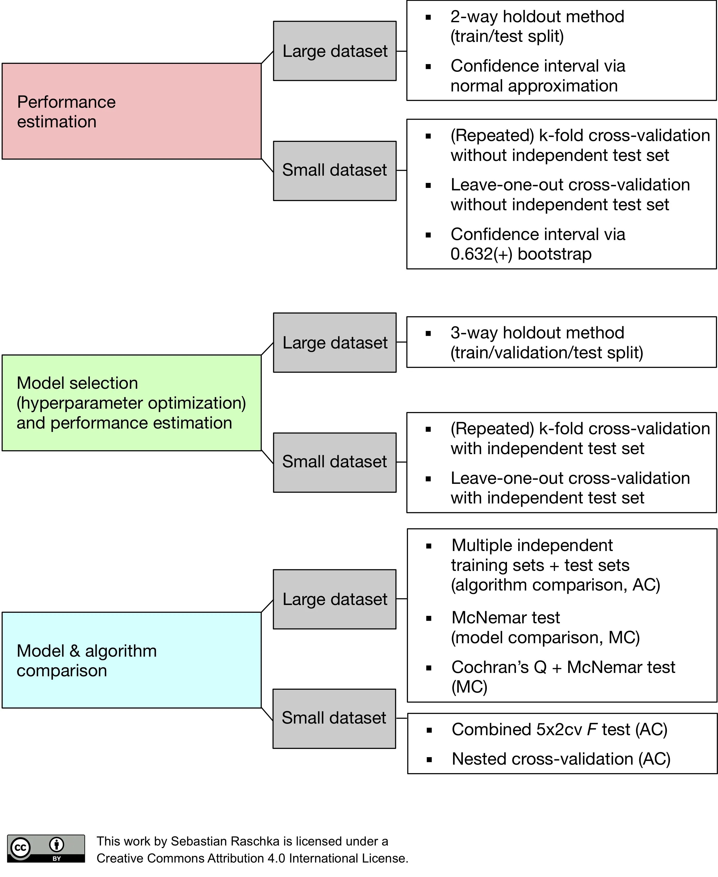 Model evaluation, model selection, and algorithm selection in machine learning
Part 4 of the model evaluation series explaining statistical tests, algorithm comparisons, corrected resampled tests, and nested cross-validation.
Model evaluation, model selection, and algorithm selection in machine learning
Part 4 of the model evaluation series explaining statistical tests, algorithm comparisons, corrected resampled tests, and nested cross-validation.
 Generating Gender-Neutral Face Images with Semi-Adversarial Neural Networks to Enhance Privacy
I thought that it would be nice to have short and concise summaries of recent projects handy, to share them with a more general audience, including...
Generating Gender-Neutral Face Images with Semi-Adversarial Neural Networks to Enhance Privacy
I thought that it would be nice to have short and concise summaries of recent projects handy, to share them with a more general audience, including...

If you read the book and have a few minutes to spare, I'd really appreciate a brief review. It helps us authors a lot!
Your support means a great deal! Thank you!