
Why do many modern LLMs use RMSNorm instead of LayerNorm?
Many modern LLMs use RMSNorm because it retains the activation-rescaling part of LayerNorm while omitting mean centering. This saves one reduction across the hidden dimension and usually removes one learned bias vector. The resulting speedup for a complete model is workload dependent, but RMSNorm has worked well in many large pre-norm transformers.
Both methods normalize each token independently across its hidden features. They do not compute statistics across tokens in the sequence or examples in the batch. For a hidden vector \(x \in \mathbb{R}^d\), LayerNorm first computes
\[\mu = \operatorname{mean}(x)\]and then applies
\[\operatorname{LayerNorm}(x) = \gamma \odot \frac{x-\mu} {\sqrt{\operatorname{mean}((x-\mu)^2)+\epsilon}} +\beta.\]Before the learned scale \(\gamma\) and shift \(\beta\), the output has approximately zero mean and unit variance. RMSNorm instead computes
\[\operatorname{RMSNorm}(x) = \gamma \odot \frac{x} {\sqrt{\operatorname{mean}(x^2)+\epsilon}}.\]It scales the root-mean-square magnitude to approximately one, but the output is generally not centered at zero. A typical RMSNorm layer has a learned scale \(\gamma\) and no learned shift. For model width \(d\), that means \(d\) affine parameters rather than the \(2d\) parameters in the common LayerNorm formulation. This parameter saving is tiny relative to the weight matrices in an LLM.
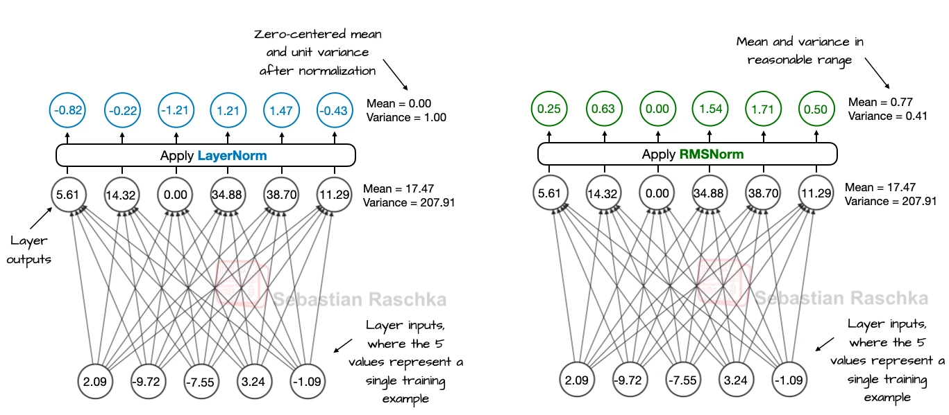
The following table summarizes the practical distinction.
| Property | LayerNorm | RMSNorm |
|---|---|---|
| Subtracts the feature mean | Yes | No |
| Divides by | Standard deviation | Root-mean-square magnitude |
| Usual learned parameters | Scale and shift | Scale |
| Unchanged by adding one constant to every feature, before the affine step | Yes | No |
| Insensitive to a positive rescaling of the whole vector, apart from \(\epsilon\) | Yes | Yes |
The shift behavior is easier to see with a small example. Suppose \(x=[1,2,3]\). LayerNorm first subtracts the mean, producing \([-1,0,1]\), and then divides by the standard deviation. Adding 10 to every entry produces the same centered values. RMSNorm keeps the positive offset. Before applying \(\gamma\), its normalized vector is approximately \([0.463, 0.926, 1.389]\). Adding 10 changes all three values after RMS normalization.
This difference is sometimes described in terms of invariance. LayerNorm removes a uniform shift across the features and normalizes their scale. RMSNorm normalizes the scale but retains information about the vector’s mean. The empirical success of RMSNorm suggests that explicit re-centering is often unnecessary in current decoder-only training recipes.
RMSNorm’s computation is also a little simpler. LayerNorm needs the mean and the mean squared deviation, followed by subtraction and division. RMSNorm only needs the mean of the squared values before division. Fused GPU kernels can make either operation fast, so the saved work should not be interpreted as a large guaranteed reduction in end-to-end training or inference time. Attention and feed-forward matrix multiplications still account for most of the computation.
In mixed-precision implementations, the squared values and their mean are often computed in float32 before the result is cast back to the input dtype. This reduces the risk of overflow and accumulated rounding error. The small \(\epsilon\) in the denominator prevents division by zero and also means the scale invariance is approximate for very small inputs.
Normalization type and normalization placement are separate architecture choices. GPT-2 uses LayerNorm before its attention and feed-forward sublayers. Llama uses RMSNorm in similar pre-norm positions. Other architectures place RMSNorm after a sublayer or add separate normalization to queries and keys inside attention. Those placement decisions change the residual path and should be evaluated independently from the LayerNorm-versus-RMSNorm choice.
The popularity of RMSNorm therefore supports a modest conclusion. It is simpler, slightly cheaper, and has been stable in successful Llama-style training recipes. It does not establish that RMSNorm always produces a better model. Architecture comparisons usually change normalization together with position embeddings, feed-forward layers, attention variants, optimizer settings, and training data. A controlled ablation is needed to attribute a quality difference to RMSNorm alone.
For the broader architecture context, see What architectural changes turned GPT-style models into Llama-style models? and How do architectures such as GPT, Llama, Qwen, and Gemma differ at a high level?.