What are some of the common ways to reduce overfitting in neural networks through model or training loop modifications?
Regularization
We can interpret regularization as a penalty against complexity. Classic regularization techniques for neural networks include L2 regularization and the related weight decay method. We implement L2 regularization by adding a penalty term to the loss function that is minimized during training. This added term represents the size of the weights, for instance, the squared sum of the weights.
Dropout reduces overfitting by randomly setting some of the activations of the hidden units to zero during training. Consequently, the neural network cannot rely on particular neurons to be activated and learns to use a larger number of neurons and learn multiple independent representations of the same data, which helps to reduce overfitting.
In early stopping, we monitor the model’s performance on a validation set during training. And we stop the training process when the performance on the validation set begins to decline.
Smaller models
Classic bias-variance theory suggests that reducing model size can reduce overfitting. The intuition behind it is that, as a general rule of thumb, the smaller the smaller the number of model parameters, the smaller its capacity to memorize or overfit to noise in the data.
Pruning. Besides reducing the number of layers and shrinking the layers’ widths as a hyperparameter tuning procedure, one approach to obtaining smaller models is iterative pruning. In iterative pruning, we train a large model to achieve the good performance on the original dataset. Then, we iteratively remove parameters of the model, retraining it on the dataset such that it maintains the same predictive performance as the original model. Iterative pruning is used in the lottery ticket hypothesis.
Knowledge distillation. Another common approach to obtaining smaller models is knowledge distillation. The general idea behind knowledge distillation is that we transfer knowledge from a large, more complex model (called teacher) to a smaller model (called student). Ideally, the student achieves the same predictive accuracy as the teacher while being more efficient due to the smaller size. And, as a nice side-effect, the smaller student may overfit less than the larger teacher model.
Ensemble methods
Ensemble methods combine predictions from multiple models to improve the overall prediction performance. However, the downside of using multiple models is an increased computational cost.
We can think of ensemble methods as asking a committee of experts: members in a committee often have different backgrounds and experiences. While they tend to agree on basic decisions, they can overrule bad decisions by majority rule. This doesn’t mean that the majority of experts is always right, but there is a good chance that the majority of the committee is more often right, on average, than every single member.
Ensemble methods are more prevalent in classical machine learning than deep learning because it is more computationally expensive to employ multiple models than relying on a single one. Or in other words, deep neural networks require significant computational resources, making them less suitable for ensemble methods. (It’s worth noting that while we previously discussed Dropout as a regularization technique, it can also be considered an ensemble method that approximates a weighted geometric mean of multiple networks.)
Popular examples of ensemble methods are random forests and gradient boosting. However, using majority voting or stacking, for example, we can combine any group of models: an ensemble may consist of a support vector machine, a multilayer perceptron, and a nearest neighbor classifier.
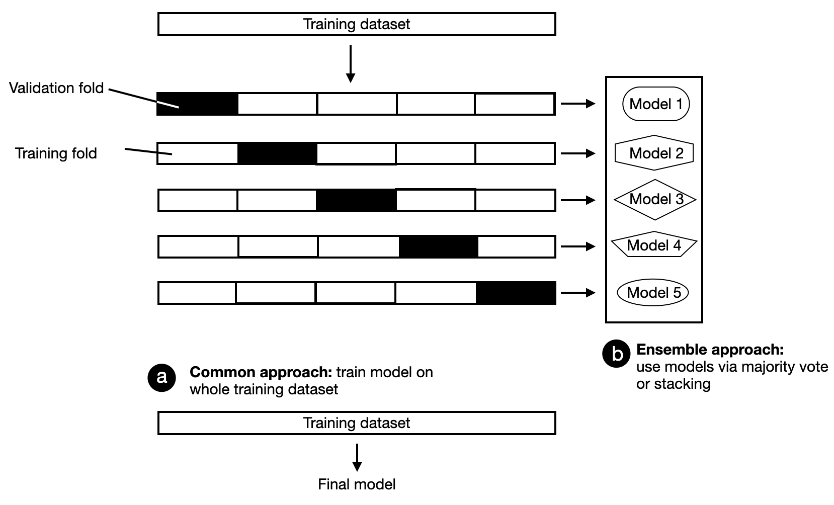
A popular technique that is often used in industry is to build models from k-fold cross-validation. K-fold cross-validation is a model evaluation technique where we train and evaluate a model on k training folds. We then compute the average performance metric across all k iterations to estimate the overall performance measure of the model. After evaluation, we can train the model on the entire training dataset, or the individual models can be combined as an ensemble, as shown in the figure below.
Other methods
The non-exhaustive list above includes the most prominent examples of techniques to reduce overfitting. Additional techniques that can reduce overfitting are skip-connections (for example, found in residual networks), look-ahead optimizers, stochastic weight averaging, multitask learning, and snapshot ensembles.
This is an abbreviated answer and excerpt from my book Machine Learning Q and AI, which contains a more verbose version with additional references and illustrations.