Machine Learning FAQ

Yes, this is definitely possible.

Let’s briefly recapitulate the concept behind Naive Bayes: Our objective function is to maximize the posterior probability given the training data:

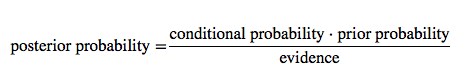
Let

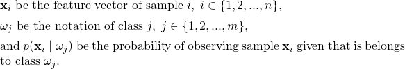
And based on the objective function, we can formulate the decision rule as:

In the context of this question, let’s not worry about the priors for now; these are typically computed via Maximum Likelihood Estimation (MLE), for instance, the class frequency N_ωj/N (number of samples in class ω_j divided by the number of all samples in the training set).

A short note about the evidence term: I wrote it for completeness, but we can simple cancel it from the decision function, because it is a constant term for all classes. Now, the class-conditional probabilities, let’s call them likelihoods, are computed as the product of the likelihoods of the individual features d:

Here, we make the “naive” conditional independence assumption, which states that features are independent of each other – that’s how Naive Bayes got its name. What we are basically saying is “The probability of observing this combination of features is equal to the product of observing each feature separately.”

Another assumption that we make is that p(x_i = b | ω_j ) is drawn from a particular distribution – that’s why Naive Bayes is also called a “generative model.” To come back to the original question, let us consider the multi-variate Bernoulli model for binary features and the Gaussian Naive Bayes model for continuous features.

The (Multi-variate) Bernoulli Model

We use the Bernoulli distribution to compute the likelihood of a binary variable. For example, we could estimate P(x_k=1 | ω_j) via MLE as the frequency of occurrences in the training set: θ = P̂(x_k=1 | ω_j) = N_{xk, ωj} / N _ωj
which reads “number of training samples in class ω_j that have the property x_k=1 (N_{xk, ωj}) divided by by all training samples in ω_j</sub> (N _ωj).” In context of text classification, this is basically the set of documents in class ω_j that contain a particular word divided by all documents in ω_j. Now, we can compute the likelihood of the binary feature vector x given class ω_j as

The Gaussian Model

Typically, we use the Gaussian Naive Bayes model for variables on a continuous scale – assuming that our variables are normal distributed.

In the equation above, we have 2 parameters we need to estimate, the mean μ of the samples associated with class ω_j and the variance σ² associated with class ω_j, respectively. This should be straight-forward, so let’s skip the details here. After we plugged the estimated parameters into the equation, we can compute the likelihood of a continuous feature vector as (similar to the Bernoulli model above).

Since we have the conditional independence assumption in Naive Bayes, we see that mixing variables is not a problem. We can compute the likelihoods of binary variables via Bernoulli Bayes and compute the likelihoods of the continuous variables via the Gaussian model. To compute the class-conditional probability of a sample, we can simply form the product of the likelihoods from the different feature subsets:

(The same concept applies to Multinomial Naive Bayes and other models.)

If you like this content and you are looking for similar, more polished Q & A’s, check out my new book Machine Learning Q and AI.