What is the decision boundary for Naive Bayes?
The decision boundary depends on the Naive Bayes variant. Gaussian Naive Bayes generally produces a quadratic boundary between two classes. Multinomial Naive Bayes produces a linear boundary in the input count features.
Why Gaussian boundaries can curve
Gaussian Naive Bayes fits a mean and variance for each feature within each class. Its log probability contains squared distances from those means. Comparing the scores for two classes therefore gives a quadratic equation in the features. If each feature has the same variance in both classes, the quadratic terms cancel and the boundary becomes linear.
With several classes, the predicted regions are formed from these pairwise comparisons. Multinomial Naive Bayes instead sums feature counts multiplied by class-specific log probabilities, plus a log prior. Those scores are linear in the counts. The scikit-learn Naive Bayes guide gives the probability models behind both variants.
Wine dataset example
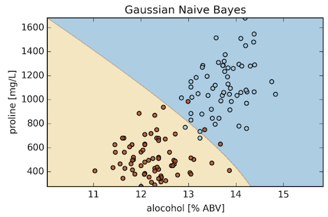
In this two-feature view of the UCI Wine dataset, the curve separates regions assigned to the two classes. Some points fall on the other side of the boundary because the fitted distributions overlap.
XOR example
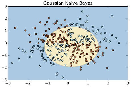
The XOR example illustrates a limitation. The class depends on a combination of features, while Naive Bayes assumes the features are conditionally independent given the class. A curved boundary alone is not enough to represent that relationship. In this sample, Gaussian Naive Bayes fits an approximately elliptical region and misclassifies many points.