Machine Learning FAQ

Gradient Descent (GD) Optimization

Using the Gradient Decent optimization algorithm, the weights are updated incrementally after each epoch (= pass over the training dataset).

The magnitude and direction of the weight update is computed by taking a step in the opposite direction of the cost gradient

where \(\eta\) is the learning rate. The weights are then updated after each epoch via the following update rule:

where \(\Delta\mathbf{w}\) is a vector that contains the weight updates of each weight coefficient \({w}\), which are computed as follows:

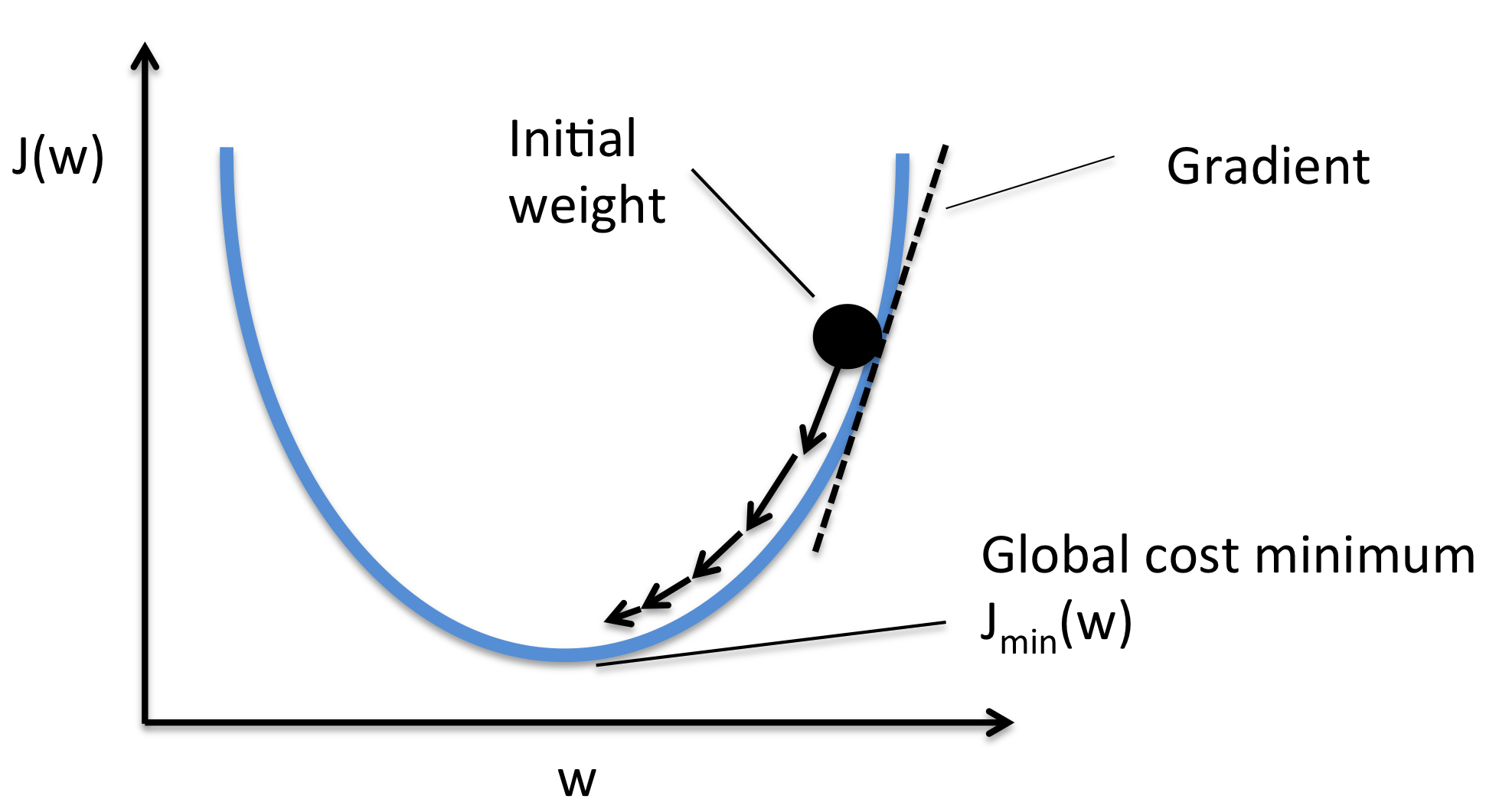
Essentially, we can picture Gradient Descent optimization as a hiker (the weight coefficient) who wants to climb down a mountain (cost function) into valley (cost minimum), and each step is determined by the steepness of the slope (gradient) and the leg length of the hiker (learning rate). Considering a cost function with only a single weight coefficient, we can illustrate this concept as follows:

Stochastic Gradient Descent (SGD)

In Gradient Descent optimization, we compute the cost gradient based on the complete training set; hence, we sometimes also call it batch gradient descent. In case of very large datasets, using Gradient Descent can be quite costly since we are only taking a single step for one pass over the training set – thus, the larger the training set, the slower our algorithm updates the weights and the longer it may take until it converges to the global cost minimum (note that the SSE cost function is convex).

In Stochastic Gradient Descent (sometimes also referred to as iterative or on-line gradient descent), we don’t accumulate the weight updates as we’ve seen above for Gradient Descent:

• for one or more epochs:
  • for each weight \(j\)
    • \(w_j := w + \Delta w_j\), where: \(\Delta w_j= \eta \sum_i (\text{target}^{(i)} - \text{output}^{(i)})x_{j}^{(i)}\)

Instead, we update the weights after each training sample:

• for one or more epochs, or until approx. cost minimum is reached:
  • for training sample \(i\):
    • for each weight \(j\)
      • \(w_j := w + \Delta w_j\), where: \(\Delta w_j= \eta (\text{target}^{(i)} - \text{output}^{(i)})x_{j}^{(i)}\)

Here, the term “stochastic” comes from the fact that the gradient based on a single training sample is a “stochastic approximation” of the “true” cost gradient. Due to its stochastic nature, the path towards the global cost minimum is not “direct” as in Gradient Descent, but may go “zig-zag” if we are visuallizing the cost surface in a 2D space. However, it has been shown that Stochastic Gradient Descent almost surely converges to the global cost minimum if the cost function is convex (or pseudo-convex)[1].

Stochastic Gradient Descent Shuffling

There are several different flavors of stochastic gradient descent, which can be all seen throughout the literature. Let’s take a look at the three most common variants:

A)

• randomly shuffle samples in the training set
  • for one or more epochs, or until approx. cost minimum is reached
    • for training sample i
      • compute gradients and perform weight updates

B)

• for one or more epochs, or until approx. cost minimum is reached
  • randomly shuffle samples in the training set
    • for training sample i
      • compute gradients and perform weight updates

C)

• for iterations t, or until approx. cost minimum is reached:
  • draw random sample from the training set
    • compute gradients and perform weight updates

In scenario A [3], we shuffle the training set only one time in the beginning; whereas in scenario B, we shuffle the training set after each epoch to prevent repeating update cycles. In both scenario A and scenario B, each training sample is only used once per epoch to update the model weights.

In scenario C, we draw the training samples randomly with replacement from the training set [2]. If the number of iterations t is equal to the number of training samples, we learn the model based on a bootstrap sample of the training set.

Mini-Batch Gradient Descent (MB-GD)

Mini-Batch Gradient Descent (MB-GD) a compromise between batch GD and SGD. In MB-GD, we update the model based on smaller groups of training samples; instead of computing the gradient from 1 sample (SGD) or all n training samples (GD), we compute the gradient from \(1 < k < n\) training samples (a common mini-batch size is \(k=50\)).

MB-GD converges in fewer iterations than GD because we update the weights more frequently; however, MB-GD let’s us utilize vectorized operation, which typically results in a computational performance gain over SGD.

Learning Rates

• An adaptive learning rate \(\eta\): Choosing a decrease constant d that shrinks the learning rate over time: \(\eta(t+1) := \eta(t) / (1 + t \times d)\)

• Momentum learning by adding a factor of the previous gradient to the weight update for faster updates: \(\Delta \mathbf{w}_{t+1} := \eta \nabla J(\mathbf{w}_{t+1}) + \alpha \Delta {w}_{t}\)

References

• [1] Bottou, Léon (1998). “Online Algorithms and Stochastic Approximations”. Online Learning and Neural Networks. Cambridge University Press. ISBN 978-0-521-65263-6
• [2] Bottou, Léon. “Large-scale machine learning with stochastic gradient descent.” Proceedings of COMPSTAT’2010. Physica-Verlag HD, 2010. 177-186.
• [3] Bottou, Léon. “Stochastic gradient descent tricks.” Neural Networks: Tricks of the Trade. Springer Berlin Heidelberg, 2012. 421-436.

If you like this content and you are looking for similar, more polished Q & A’s, check out my new book Machine Learning Q and AI.