How to compute gradients with backpropagation for arbitrary loss and activation functions?
Backpropagation is basically “just” clever trick to compute gradients in multilayer neural networks efficiently. Or in other words, backprop is about computing gradients for nested functions, represented as a computational graph, using the chain rule. Backpropagation includes computational tricks to make the gradient computation more efficient, i.e., performing the matrix-vector multiplication from “back to front” and storing intermediate values (or gradients). Hence, backpropagation is a particular way of applying the chain rule, in a certain order, to speed things up.
In other words, backprop is about computing the chain rule backwards, that is, given something like,
\[\frac{\partial A}{ \partial D} =\frac{\partial A}{ \partial B} \frac{\partial B}{ \partial C} \frac{\partial C}{ \partial D},\]starting by computing
\[\frac{\partial B}{ \partial C} \frac{\partial C}{ \partial D}\]rather than starting by computing
\[\frac{\partial A}{ \partial B} \frac{\partial B}{ \partial C}.\]This has efficiency implications since the output of a neural network is a vector, whereas the inputs and hidden activation values are stored in matrices. And multiplying a matrix by a matrix is more expensive than multiplying a matrix with a vector (where a vector means \(\mathbb{R}^{n \times 1}\) matrix in this context).
In multilayer neural networks, it is a common convention to, e.g., tie a logistic sigmoid unit to a cross-entropy (or negative log-likelihood) loss function; however, this choice is essentially arbitrary. We can mix and match cost and activation functions as we like since all we care about is computing the gradient of the loss with respect to the weight parameters in the different layers to perform a gradient-based update of the weights.
Single-layer neural network/logistic regression example
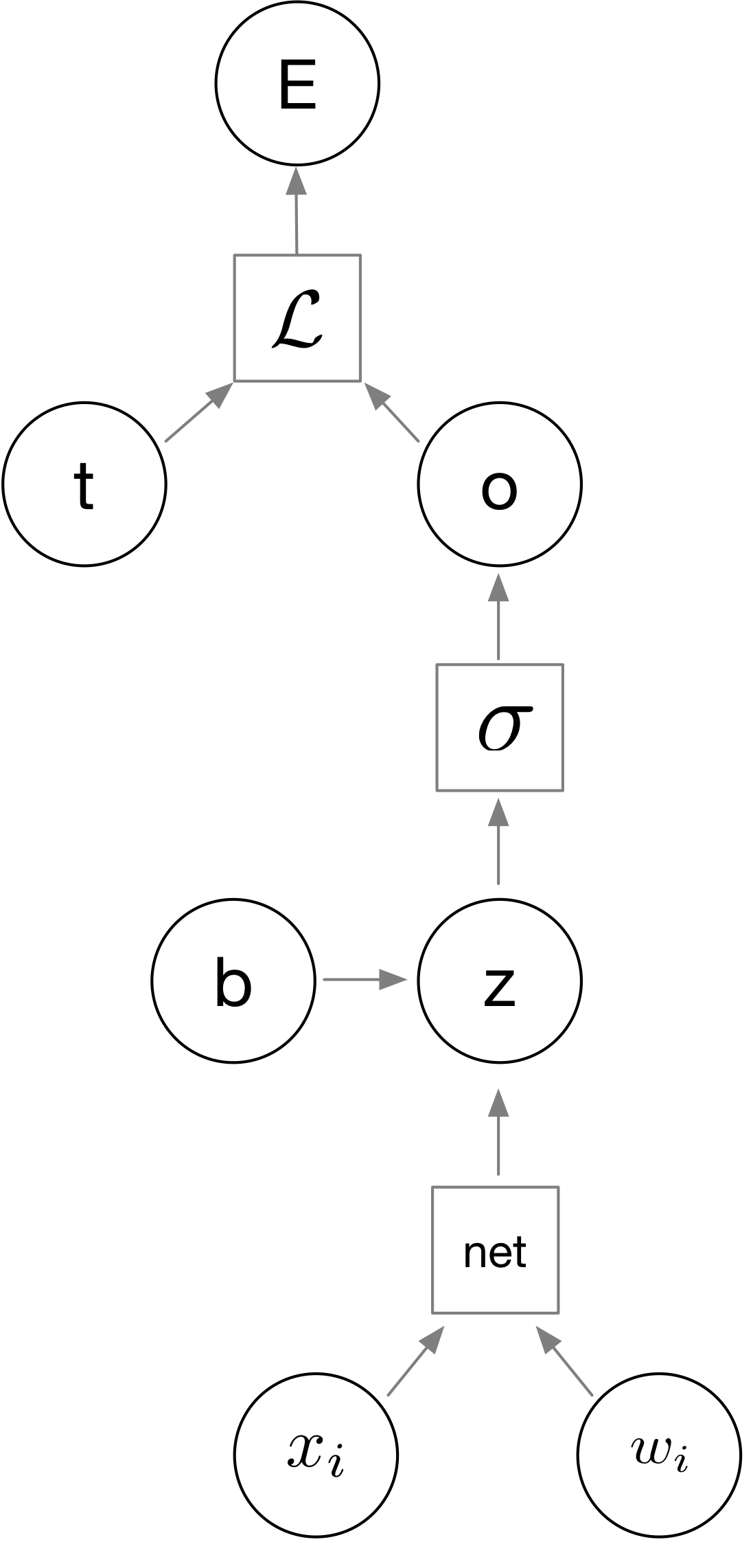
For example, let’s assume we want to use gradient descent to update the weights in a single-layer neural network with respect to an error E computed by the loss function \(\mathcal{L}\), as illustrated in the next figure.
Here, as a warm up for simplicity, let’s consider \(w_i\) the \(i\)th weigth parameter in a single layer neural network. Further, let
- \(w_i\) is the weight parameter we want to update with respect to the error E,
-
\(x_i\) the network input,
- \(\sigma(\cdot)\) be the activation function to compute an activation value \(a\),
- \(x\) be an input value,
- \(b\) the bias unit,
- \(z\) is the variable computed by the “net,” function, the weighted sum of the inputs \(\sum_i w_i x_i\),
- $o$ the output value,
- and $t$ the target value we want to predict (e.g., class label).
In short, our goal is to compute the gradient
\[\frac{\partial E}{\partial w_i},\]to update the weight parameter \(w_i\):
\[\frac{\partial E}{\partial w_i} = \frac{\partial E}{\partial o} \frac{\partial o}{\partial z} \frac{\partial z}{\partial w}\]If the error is computed via the mean squared error,
\[\mathcal{L(o, t)} =E = \frac{1}{2m} \sum_j(t_j-o_j)^ 2,\]we would arrive at the following:
\[\begin{align} \frac{\partial E}{w_i} = -\frac{1}{m} \sum_j (t_j - o_j) \frac{\partial o_i}{\partial \text{net}_i} \frac{\partial \text{net}_i}{\partial w_i}. \end{align}\]- For how to derive the mean squared error loss, \(\frac{\partial E}{\partial o}\), with respect to the network’s output, see the the related FAQ entry What is the derivative of the Mean Squared Error?
The derivative $\frac{\partial o_i}{\partial \text{net}_i}$ that is used to compute the output ($o$) depends on what kind of acivation function we use. If it is a logistic sigmoid function \(\sigma\), it is \((1 - \sigma(z)) \sigma(z)\) as explained in more detail in the related FAQ entry What is the derivative of the logistic sigmoid function?
Together with the simple derivative
\[\frac{\partial \text{net}_i}{\partial w_i} = x_i,\]we can put it all together as
\[\begin{align} \frac{\partial E}{w_i} &= -\frac{1}{m} \sum_j (t_j - o_j) \frac{\partial o_i}{\partial \text{net}_i} \frac{\partial \text{net}_i}{\partial w_i} \\ & = -\frac{1}{m} \sum_j (t_j - o_j) o_j(1-o_j)x_j. \end{align}\]So, while the above illustrated the concept of backpropagation on a single-layer neural network, we can extend this concept to multiple layers. For instance, consider the case of a multilayer neural network with one hidden layer. The changes compared to the 1-layer variant are highlighted in red. Basically, if you compare the single to the multi-layer variant below, you can see that I just copy&pasted the middle part and add indices (1) and (2) to the weights, activation units etc.:
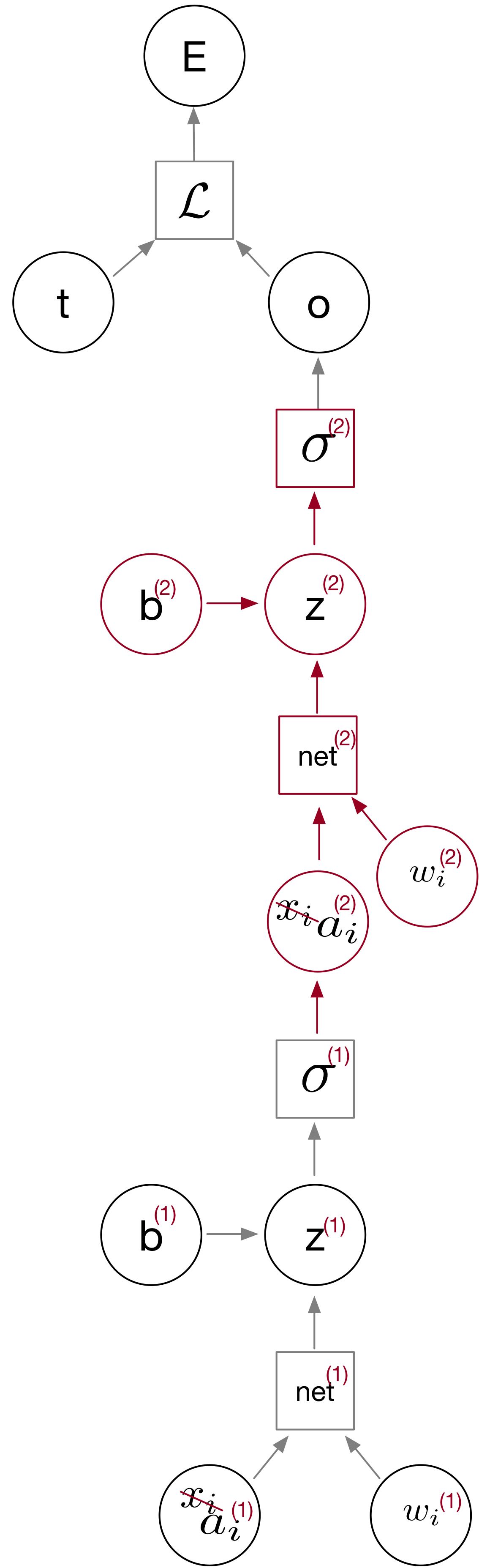
So, in this case, we want to compute the gradients of the weights in the “first” layer ($w^{(1)}$) and second layer ($w^{(2)}$). For instance,
the equation we defined earlier,
\[\frac{\partial E}{\partial w_i} = \frac{\partial E}{\partial o} \frac{\partial o}{\partial z} \frac{\partial z}{\partial w},\]
can be used to compute the hidden layer weights:
\(\frac{\partial E}{\partial w_i^{(2)}} = \frac{\partial E}{\partial o} \frac{\partial o}{\partial z^{(2)}} \frac{\partial z^{(2)}}{\partial w^{(2)}}.\) And the input layer gradients can be computed similarly,
\[\frac{\partial E}{\partial w_i^{(1)}} = \frac{\partial E}{\partial o} \frac{\partial o}{\partial z^{(2)}} \frac{\partial z^{(2)}}{\partial a^{(2)}}\frac{\partial a^{(2)}}{\partial z^{(1)}}\frac{\partial z^{(1)}}{\partial w_j^{(1)}}.\]Note that a part of the “backprop” algorithm (versus the standard chain rule concept) is that we save intermediate values from earlier layers to compute the gradients of later layers (here: \(\frac{\partial E}{\partial o} \frac{\partial o}{\partial z^{(2)}}\)).
In any case, the bottom line is that you just need to compute the individual components above, which depend on the loss and activation functions of your choice.