Noteworthy LLM Research Papers of 2024

I hope your 2025 is off to a great start! To kick off the year, I’ve finally been able to complete the draft of this AI Research Highlights of 2024 article. It covers a variety of topics, from mixture-of-experts models to new LLM scaling laws for precision.

Reflecting on all the major research highlights of 2024 would probably require writing an entire book. It’s been an extraordinarily productive year, even for such a fast-moving field. To keep things reasonably concise, I decided to focus exclusively on LLM research in this article. But even then, how does one choose a subset of papers from such an eventful year? The simplest approach I could think of was to highlight one paper per month: January through December 2024.

So, in this article, I’ll share 12 research highlights—papers that I personally found fascinating, impactful, or, ideally, both.

The selection criteria are admittedly subjective, based on what stood out to me this year. I’ve also aimed for some variety, so it’s not all just about LLM model releases.

If you’re looking for a broader list of AI research papers, feel free to check out my earlier article (LLM Research Papers: The 2024 List).

Happy new year and happy reading!

Table of contents

• 1. January: Mixtral’s Mixture of Experts Approach
  • 1.1 Understanding MoE models
  • 1.2  The relevance of MoE models today
• 2. February: Weight-decomposed LoRA
  • 2.2 LoRA Recap
  • 2.2 From LoRA to DoRA
  • 2.3 The future of LoRA and LoRA-like methods
• 3. March: Tips for Continually Pretraining LLMs
  • 3.1 Simple techniques work
  • 3.2 Will these simple techniques continue to work?
• 4. April: DPO or PPO for LLM alignment, or both?
  • 4.1 RLHF-PPO and DPO: What Are They?
  • 4.2 PPO Typically Outperforms DPO
  • 4.3 How are PPO and DPO used today?
• 5. May: LoRA learns less and forgets less
  • 5.1 LoRA learns less
  • 5.2 LoRA forgets less
  • 5.3 The LoRA trade-off
  • 5.4 Future ​approaches to finetuning LLMs
• 6. June: The 15 Trillion Token FineWeb Dataset
  • 6.1 Comparison to other datasets
  • 6.2 Principled dataset development
  • 6.3 The relevance of FineWeb today
• 7. July: The Llama 3 Herd of Models
  • 7.1 Llama 3 architecture summary
  • 7.2 Llama 3 training
  • 7.3 Multimodal Llamas
  • 7.4 Llama 3 impact and usage
• 8. August: Improving LLMs by scaling inference-time compute
  • 8.1 Improve outputs by using more test-time computation
  • 8.2 Optimizing test-time computation techniques
  • 8.3 Test-time computation versus pretraining a larger model
  • 8.4 Future relevance of test-time compute scaling
• 9. September: Comparing multimodal LLM paradigms
  • 9.1 Multimodal LLM paradigms
  • 9.2 Nvidia’s hybrid approach
  • 9.3 Multimodal LLMs in 2025
• 10. October: Replicating OpenAI O1’s reasoning capabilities
  • 10.1 Shortcut learning vs journey learning
  • 10.2 Constructing long thoughts
  • 10.3 Distillation – the quick fix?
  • 10.4 The state of AI research
  • 10.5 The future of LLMs in the light of o1 (and o3)
• 11. November: LLM scaling laws for precision
  • 11.1 Chinchilla scaling laws refresher
  • 11.2 Low-precision training
  • 11.3 Precision scaling laws takeaways
  • 11.4 Model scaling laws in 2025
• 12. December: Phi-4 and learning from synthetic data
  • 12.1 Phi-4 performance
  • 12.2 Synthetic data learnings
  • 12.4 Future importance of synthetic data
• Conclusions and outlook
  • Multimodal LLMs
  • Computational efficiency
  • State space models
  • Scaling
  • What I am looking forward to

1. January: Mixtral’s Mixture of Experts Approach

Only a few days into January 2024, the Mistral AI team shared the Mixtral of Experts paper (8 Jan 2024), which described Mixtral 8x7B, a Sparse Mixture of Experts (SMoE) model.

The paper and model were both very influential at the time, as Mixtral 8x7B was (one of) the first open-weight MoE LLMs with an impressive performance: it outperformed Llama 2 70B and GPT-3.5 across various benchmarks.

1.1 Understanding MoE models

An MoE, or Mixture of Experts, is an ensemble model that combines several smaller “expert” subnetworks inside the GPT-like decoder architecture. Each subnetwork is said to be responsible for handling different types of tasks or, more concretely, tokens. The idea here is that by using multiple smaller subnetworks instead of one large network, MoEs aim to allocate computational resources more efficiently.

In particular, in Mixtral 8x7B, is to replace each feed-forward module in a transformer architecture with 8 expert layers, as illustrated in the figure below.

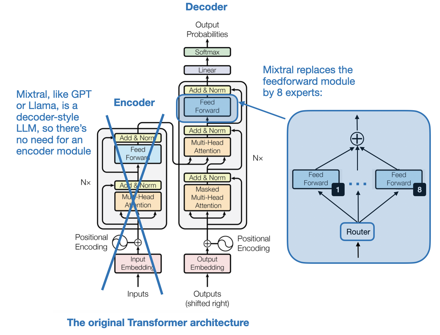
“Sparse” in the context of a “Sparse Mixture of Experts” refers to the fact that at any given time, only a subset of the expert layers (typically 1 or 2 out of the 8 in Mixtral 8x7B) are actively used for processing a token.

As illustrated in the figure above, the subnetworks replace the feed-forward module in the LLM. A feed-forward module is essentially a multilayer perceptron. In PyTorch-like pseudocode, it essentially looks like this:

class FeedForward(torch.nn.Module):

    def __init__(self, embed_dim, coef):
        super().__init__()

        self.layers = nn.Sequential(
            torch.nn.Linear(embed_dim, coef*embed_dim),
            torch.nn.ReLU(),
            torch.nn.Linear(coef*n_embed, embed_dim),
            torch.nn.Dropout(dropout)
        )

    def forward(self, x):
        return self.layers(x)

In addition, there is also a Router module (also known as a gating network) that redirects each of the token embeddings to the 8 expert feed-forward modules. The outputs from these 8 expert feed-forward layers are then summed, as illustrated in the figure below.

Since there are 11 more papers to cover in this article, I want to keep this description of the Mixtral model brief. However, you can find additional details in my previous article, “Model Merging, Mixtures of Experts, and Towards Smaller LLMs” (https://magazine.sebastianraschka.com/i/141130005/mixtral-of-experts)

1.2  The relevance of MoE models today

At the beginning of the year, I would have thought that open-weight MoE models would be more popular and widely used than they are today. While they are not irrelevant, many state-of-the-art models still rely on dense (traditional) LLMs rather than MoEs though, e.g., Llama 3, Qwen 2.5, Gemma 2, etc. However, it is, of course, impossible to say what proprietary architectures like GPT-4, Gemini, and Claude are based on; they might as well be using MoE under the hood.

In any case, MoE architectures are still relevant, especially as they offer a way to scale large language models efficiently by activating only a subset of the model’s parameters for each input, thus reducing computation costs without sacrificing model capacity.

2. February: Weight-decomposed LoRA

If you are finetuning open-weight LLMs, chances are high that you have been using low-rank adaptation (LoRA), a method for parameter-efficient LLM finetuning, at some point.

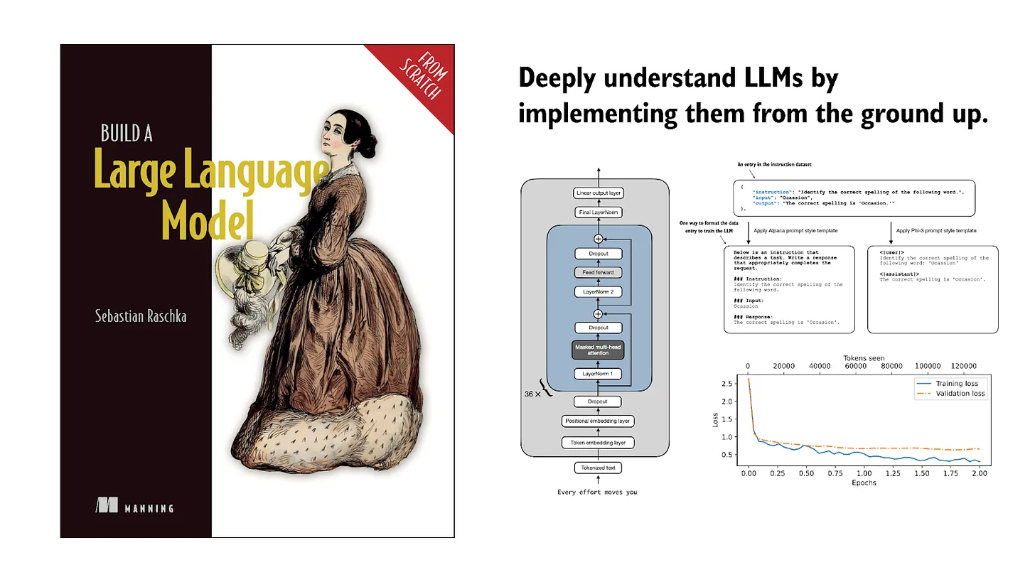
If you are new to LoRA, I have written a previous article on Practical Tips for Finetuning LLMs Using LoRA (Low-Rank Adaptation) that you might helpful, and I have a from-scratch code implementation in Appendix D of my Build A Large Language Model (From Scratch) book.

Since LoRA is such a popular and widely used method, and since I had so much fun implementing and playing with a newer variant, my pick for February is DoRA: Weight-Decomposed Low-Rank Adaptation (February 2024) by Liu and colleagues.

2.2 LoRA Recap

Before introducing DoRA, here’s a quick LoRA refresher:

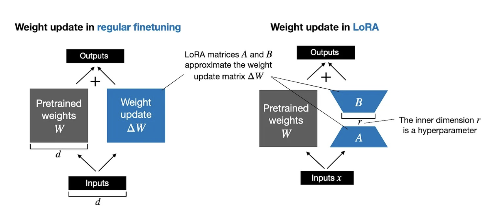
Full finetuning updates each large weight matrix W in an LLM by computing a large weight update matrix ΔW. LoRA approximates ΔW as the product of two smaller matrices A and B. So, Instead of W + ΔW, we have W + A.B. This greatly reduces computational and memory overhead.

The figure below illustrates these formulas for full finetuning and LoRA side by side.

2.2 From LoRA to DoRA

DoRA (Weight-Decomposed Low-Rank Adaptation) extends LoRA by first decomposing a pretrained weight matrix into two parts: a magnitude vector m and a directional matrix V. This decomposition is rooted in the idea that any vector can be represented by its length (magnitude) and direction (orientation), and here we apply it to each column vector of a weight matrix. Once we have m and V, DoRA applies LoRA-style low-rank updates only to the directional matrix V, while allowing the magnitude vector m to be trained separately.

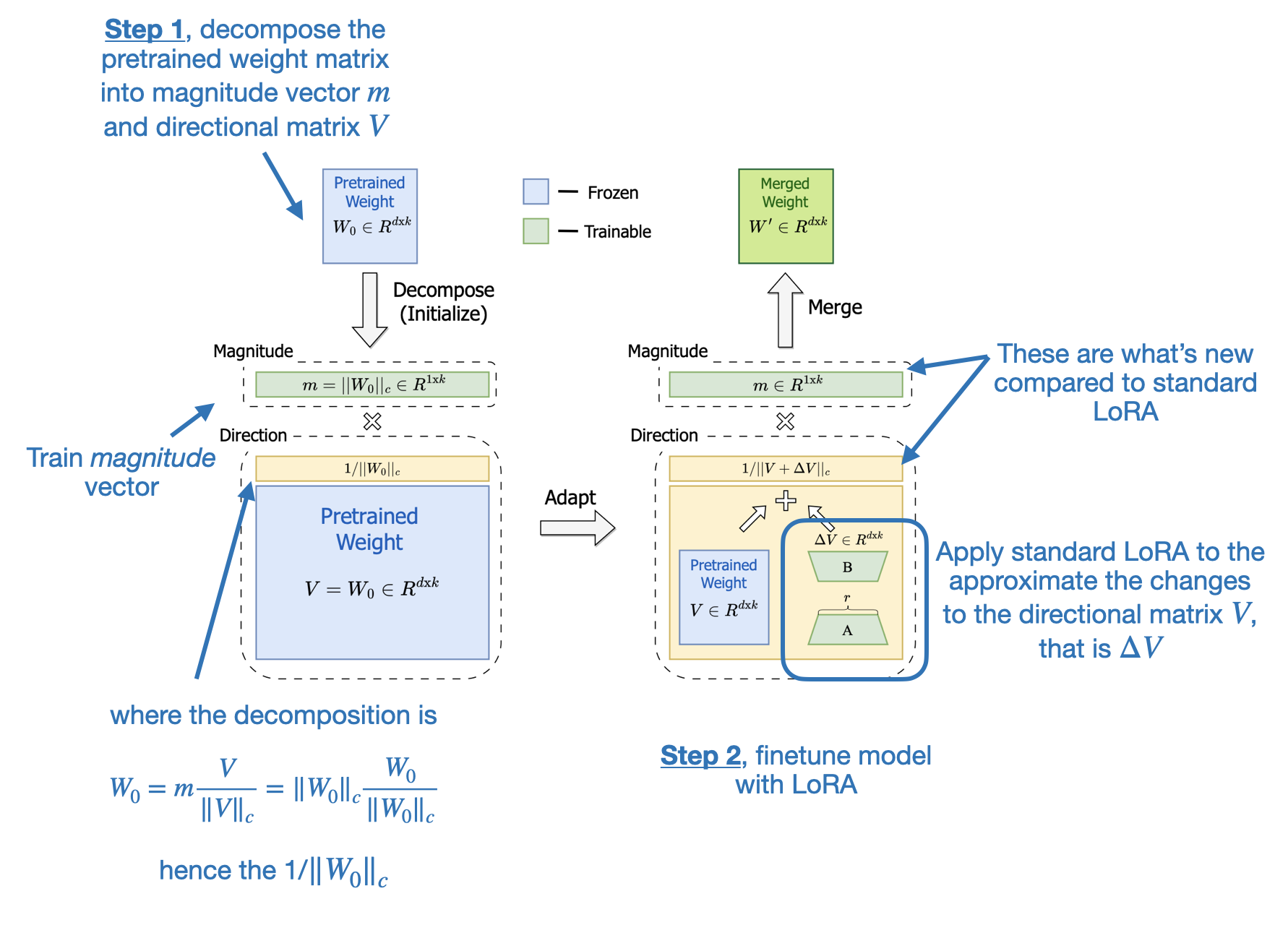
This two-step approach gives DoRA more flexibility than standard LoRA. Rather than uniformly scaling both magnitude and direction as LoRA tends to do, DoRA can make subtle directional adjustments without necessarily increasing the magnitude. The result is improved performance and robustness, as DoRA can outperform LoRA even when using fewer parameters and is less sensitive to the choice of rank.

Again, I am keeping this section brief since there are 10 more to go, but if you are interested in additional details, I dedicated a whole article to this method earlier this year: “Improving LoRA: Implementing Weight-Decomposed Low-Rank Adaptation (DoRA) from Scratch” (https://magazine.sebastianraschka.com/p/lora-and-dora-from-scratch)

2.3 The future of LoRA and LoRA-like methods

DoRA is a small, logical improvement over the original LoRA method. While it hasn’t been widely adopted yet, it adds minimal complexity and is worth considering the next time you fine-tune an LLM. In general, I expect LoRA and similar methods to remain popular. For example, Apple recently mentioned in their Apple Intelligence Foundation Language Models paper that they use LoRA for on-device task specialization of LLMs.

3. March: Tips for Continually Pretraining LLMs

As far as I can tell, instruction-finetuning is the most popular form of finetuning by LLM practitioners. The goal here is to get openly available LLMs to better follow instructions or specialize these LLMs on subsets or new instructions.

However, when it comes to taking in new knowledge, continued pretraining (sometimes also referred to continually pretraining) is the way to go.

In this section, I want to briefly summarize the refreshingly straightforward Simple and Scalable Strategies to Continually Pre-train Large Language Models (March 2024) paper by Ibrahim and colleagues.

3.1 Simple techniques work

This 24-page Continually Pre-train Large Language Models paper reports a large number of experiments and comes with countless figures, which is very thorough for today’s standards.

What were the main tips for applying continued pretraining successfully?

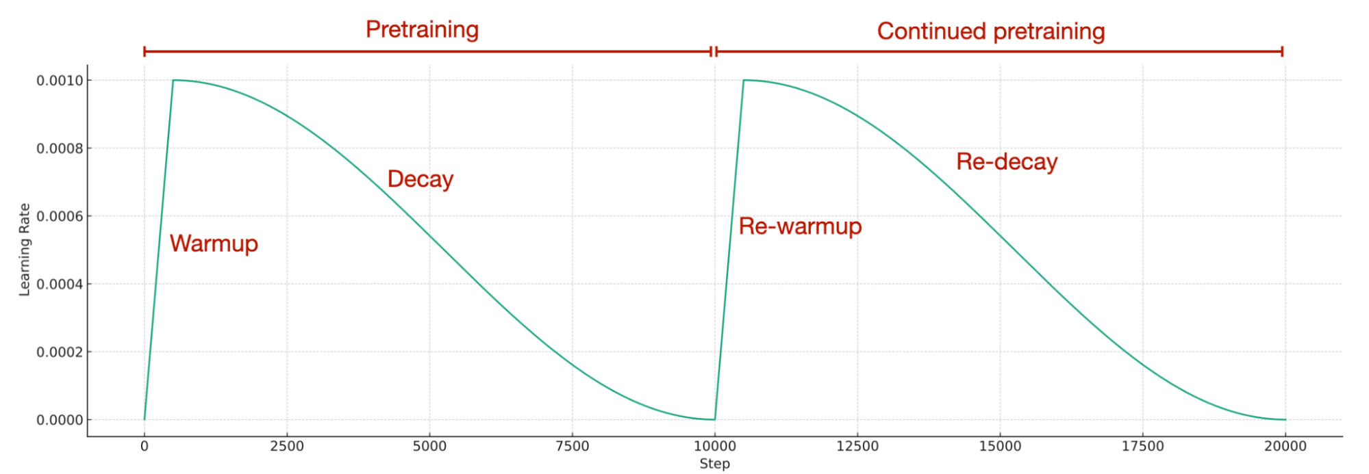
1. Simple re-warming and re-decaying the learning rate

2. Adding a small portion (e.g., 5%) of the original pretraining data (D1) to the new dataset (D2) to prevent catastrophic forgetting. Note that smaller fractions like 0.5% and 1% were also effective.

To be a bit more concrete regarding point 1, re-warming and re-decaying, this means we employ the exact same learning rate schedule that was used during the initial pretraining stage of an LLM.

As far as I know, the re-warming and re-decaying, as well as adding original pretraining data to the new data, is more or less common knowledge. However, I really appreciate that the researchers took the time to formally test this method in this very detailed 24-page report.

If you are interested in additional details, I discussed this paper more thoroughly in my previous “Tips for LLM Pretraining and Evaluating Reward Models” article (https://magazine.sebastianraschka.com/p/tips-for-llm-pretraining-and-evaluating-rms).

3.2 Will these simple techniques continue to work?

I have no reason to believe that these methods will not continue to work for future LLMs. However, it is important to note that pretraining pipelines have become more sophisticated, consisting of multiple stages, including short- and long-context pretraining. So, for optimal results, the recipes suggested in this paper may need to be tweaked under certain circumstances.

4. April: DPO or PPO for LLM alignment, or both?

April is a tough choice. For instance, Kolmogorov-Arnold Networks made a big wave that month. But as far as I can tell, the excitement fizzled out pretty quickly. This is likely because their theoretical guarantees are difficult to implement practically, they lack competitive results or benchmarks, and other architectures are much more scalable.

So, instead, my pick for April goes to a more practical paper: Is DPO Superior to PPO for LLM Alignment? A Comprehensive Study (April 2024) by Xu and colleagues.

4.1 RLHF-PPO and DPO: What Are They?

Before summarizing the paper itself, here’s an overview of Proximal Policy Optimization (PPO) and Direct Preference Optimization (DPO), both popular methods in aligning LLMs via Reinforcement Learning with Human Feedback (RLHF). RLHF is the method of choice to align LLMs with human preferences, improving the quality but also the safety of their responses.

Traditionally, RLHF-PPO has been a crucial step in training LLMs for models and platforms like InstructGPT and ChatGPT. However, DPO started gaining traction last year due to its simplicity and effectiveness. In contrast to RLHF-PPO, DPO does not require a separate reward model. Instead, it directly updates the LLM using a classification-like objective. Many LLMs now utilize DPO, although comprehensive comparisons with PPO are lacking.

Below are two resources on RLHF and DPO I developed and shared earlier this year:

• LLM Training: RLHF and Its Alternatives
• Direct Preference Optimization (DPO) for LLM Alignment (From Scratch)

4.2 PPO Typically Outperforms DPO

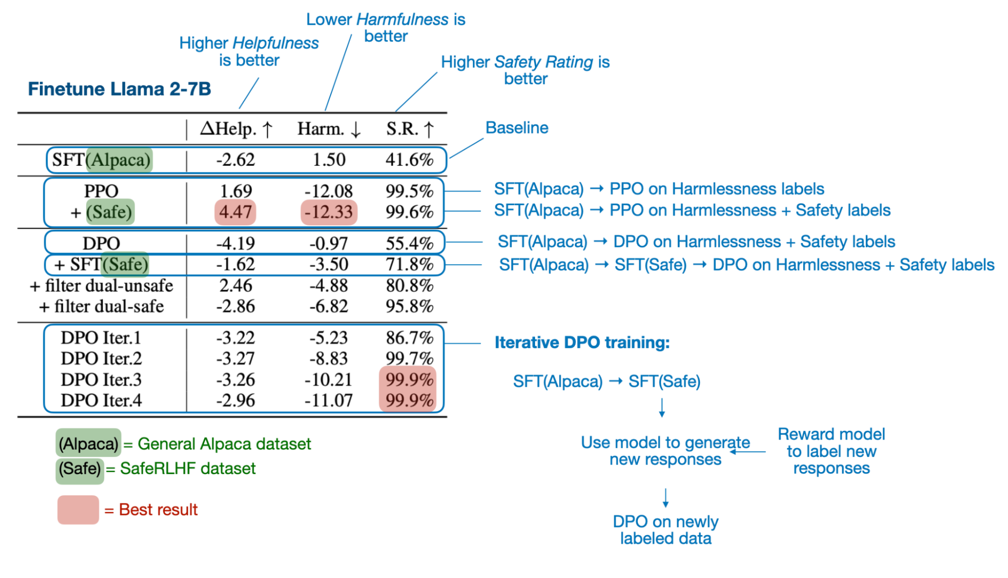
Is DPO Superior to PPO for LLM Alignment? A Comprehensive Study is a well-written paper with numerous experiments and results. The key conclusions are that PPO tends to outperform DPO, and that DPO is inferior when dealing with out-of-distribution data.

Here, out-of-distribution data means the language model was previously trained on instruction data (via supervised finetuning) that differs from the preference data used for DPO. For instance, a model might be trained on the general Alpaca dataset before undergoing DPO finetuning on a different preference-labeled dataset. (However, one way to improve DPO on such out-of-distribution data is to first conduct a supervised instruction-finetuning step using the preference dataset, and then perform DPO finetuning.)

The main findings are summarized in the figure below.

4.3 How are PPO and DPO used today?

PPO might have a slight edge when it comes to the raw modeling performance of the resulting LLM. However, DPO is much easier to implement and computationally more efficient to apply (you don’t have to train and use a separate reward model, after all). Hence, to the best of my knowledge, DPO is also much more widely used in practice than RLHF-PPO.

One interesting example is Meta AI’s Llama models. While Llama 2 was trained with RLHF-PPO, the newer Llama 3 models used DPO.

Interestingly, recent models even use both PPO and DPO nowadays. Recent examples include Apple’s Foundation Models and Allen AI’s Tulu 3.

5. May: LoRA learns less and forgets less

I found another LoRA paper this year particularly interesting (this is the last LoRA paper in this 12-paper selection, I promise!). I wouldn’t call it groundbreaking, but I really like it since it formalizes some of the common knowledge around finetuning LLMs with (and without) LoRA: LoRA Learns Less and Forgets Less (May 2024) by Biderman and colleagues.

LoRA Learns Less and Forgets Less is an empirical study comparing low-rank adaptation (LoRA) to full finetuning on large language models (LLMs), focusing on two domains (programming and mathematics) and two tasks (instruction finetuning and continued pretraining). Check out the February section above if you’d like a refresher on LoRA before proceeding.

5.1 LoRA learns less

The study shows LoRA learns noticeably less than full finetuning, especially in tasks like coding, where new knowledge needs to be acquired. The gap is smaller when only instruction finetuning is performed. This suggests that pretraining on new data (learning new knowledge) benefit more from full finetuning than converting a pretrained model into an instruction follower.

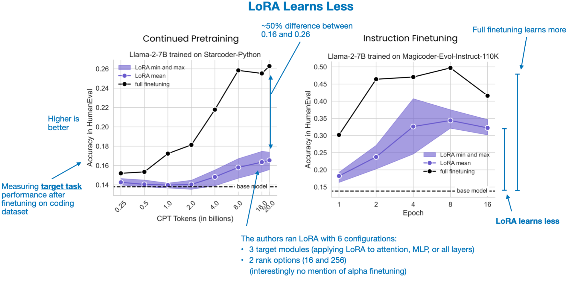
There are some more nuances, though. For math tasks, for example, the difference between LoRA and full finetuning shrinks. This may be because math problems are more familiar to the LLM, and they likely encountered similar problems during pretraining. In contrast, coding involves a more distinct domain, requiring more new knowledge. Thus, the farther a new task is from the model’s pretraining data, the more beneficial full finetuning becomes in terms of learning capacity.

5.2 LoRA forgets less

When examining how much previously acquired knowledge is lost, LoRA consistently forgets less. This is particularly clear when adapting to data far from the source domain (e.g., coding). With coding tasks, full finetuning leads to significant forgetting, while LoRA preserves more original capabilities. In math, where the model’s original knowledge was already closer to the new task, the difference is less pronounced.

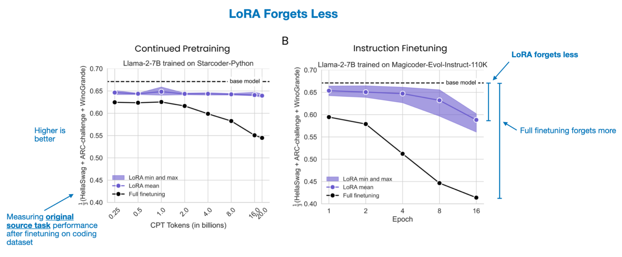
5.3 The LoRA trade-off

Overall, there is a trade-off: full finetuning is better for absorbing new knowledge from more distant domains but leads to more forgetting of previously learned tasks. LoRA, by changing fewer parameters, learns less new information but retains more of the original capabilities.

5.4 Future ​approaches to finetuning LLMs

The study primarily compares LoRA to full finetuning. In practice, LoRA has gained popularity because it is far more resource-efficient than full finetuning. In many cases, full finetuning is simply not feasible due to hardware constraints. Moreover, if you only need to address specialized applications, LoRA alone may be sufficient. Since LoRA adapters can be stored separately from the base LLM, it’s easy to preserve the original capabilities while adding new ones. Additionally, it’s possible to combine both methods by using full finetuning for knowledge updates and LoRA for subsequent specialization.

In short, I think both methods will continue to be very relevant in the upcoming year(s). It’s more about using the right approach for the task at hand.

6. June: The 15 Trillion Token FineWeb Dataset

The FineWeb Datasets: Decanting the Web for the Finest Text Data at Scale (June 2024) paper by Penedo and colleagues describes the creation of a 15 trillion token dataset for LLMs and making it publicly available, including a link to download the dataset and a code repository (datatrove/examples/fineweb.py) to reproduce the dataset preparation steps.

6.1 Comparison to other datasets

Since several other large datasets for LLM pretraining are available, what’s so special about this one? Other datasets are comparatively small: RefinedWeb (500B tokens), C4 (172B tokens), the Common Crawl-based part of Dolma 1.6 (3T tokens) and 1.7 (1.2T tokens), The Pile (340B tokens), SlimPajama (627B tokens), the deduplicated variant of RedPajama (20T tokens), English CommonCrawl section of Matrix (1.3T tokens), English CC-100 (70B tokens), Colossal-OSCAR (850B tokens).

For example, ~360 billion tokens are only suited for small LLMs (for instance, 1.7 B, according to the Chinchilla scaling laws). On the other hand, the 15 trillion tokens in the FineWeb dataset should be optimal for models up to 500 billion parameters according to the Chinchilla scaling laws. (Note that RedPajama contains 20 trillion tokens, but the researchers found that models trained on RedPajama result in poorer quality than FineWeb due to the different filtering rules applied.)

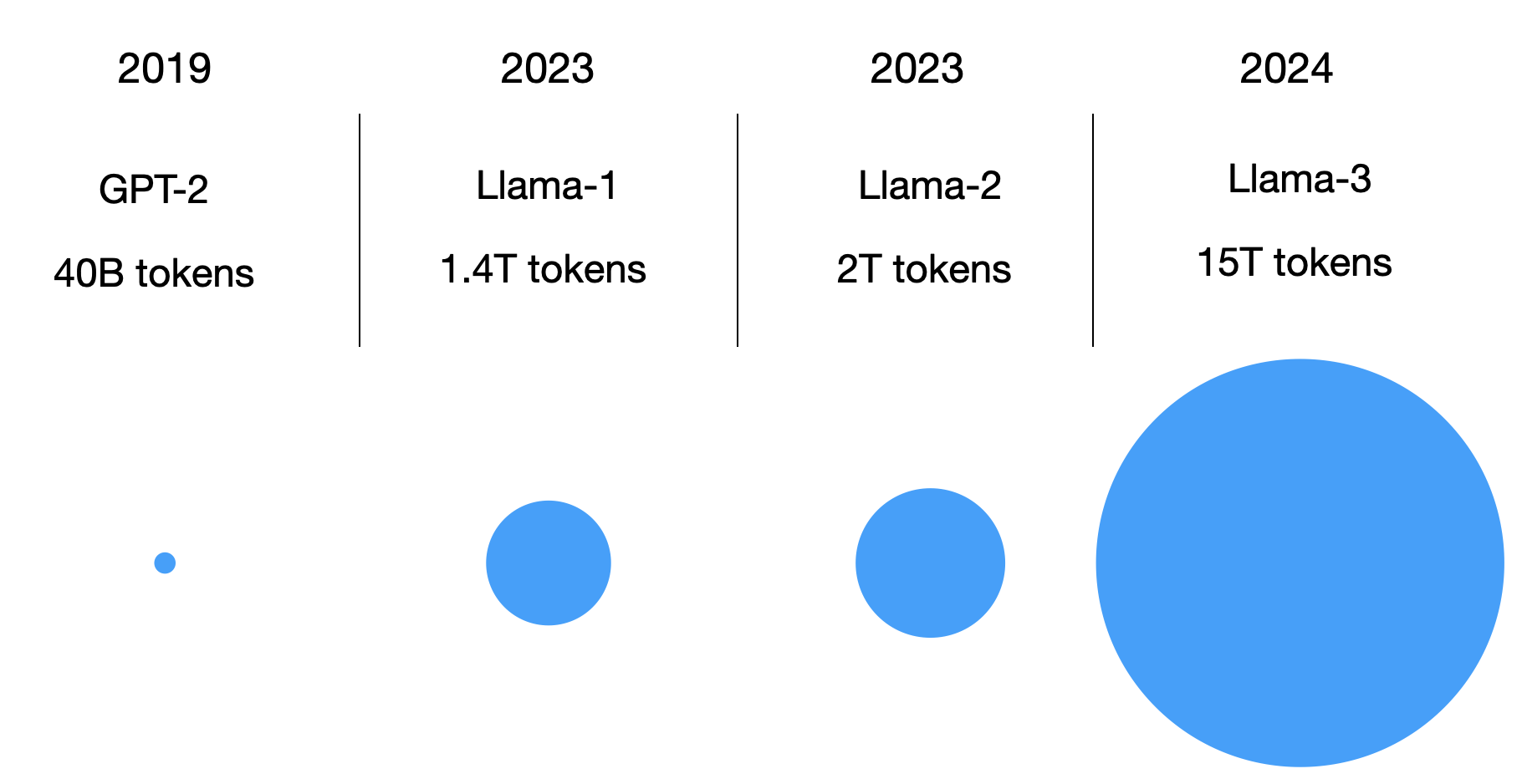
In short, the FineWeb dataset (English-only) makes it theoretically possible for researchers and practitioners to train large-scale LLMs. (Side note: The Llama 3 models with 8B, 70B, and 405B sizes were trained on 15 trillion tokens as well, but Meta AI’s training dataset is not publicly available.)

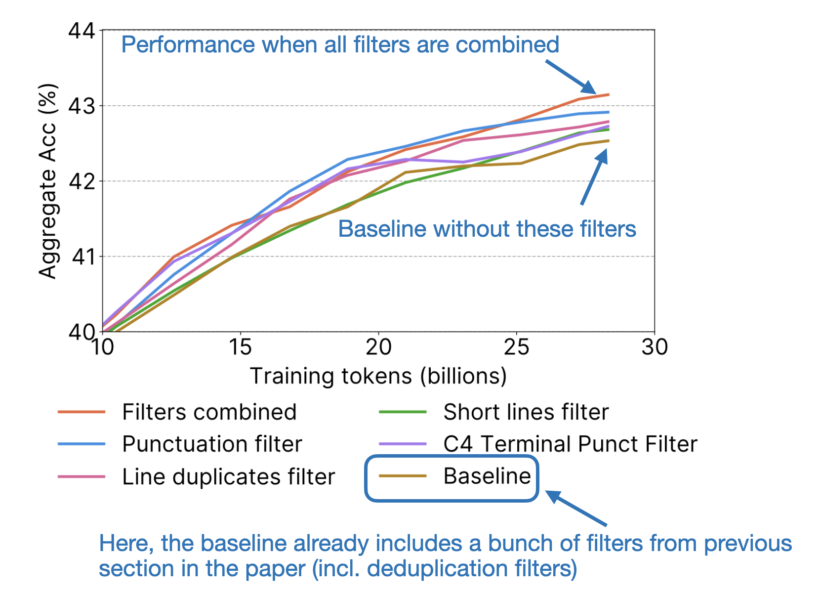
6.2 Principled dataset development

In addition, the paper contains principled ablation studies and insights into how the filtering rules were developed and applied to arrive at the FineWeb dataset (starting from the CommonCrawl web corpus). In short, for each filtering rule they tried, they took a 360 billion token random sample from the original and the filtered data and then trained a small 1.71 billion parameter Llama-like model to see whether the filtering rule is beneficial or not based on the models’ performances on standard benchmarks such as HellaSwag, ARC, MMLU, and others.

6.3 The relevance of FineWeb today

Overall, while pretraining multi-billion parameter LLMs may still be beyond the reach of most research labs and companies, this dataset is a substantial step toward democratizing the study and development of LLMs. In summary, this paper represents a commendable effort and introduces a valuable public resource for advancing pretraining in LLMs.

7. July: The Llama 3 Herd of Models

Readers are probably already well familiar with Meta AI’s Llama 3 models and paper, but since these are such important and widely-used models, I want to dedicate the July section to The Llama 3 Herd of Models (July 2024) paper by Grattafiori and colleagues.

What’s notable about the Llama 3 model family is the increased sophistication of the pre-training and post-training pipelines compared to its Llama 2 predecessor. Note that this is not only true for Llama 3 but other LLMs like Gemma 2, Qwen 2, Apple’s Foundation Models, and others, as I described a few months ago in my New LLM Pre-training and Post-training Paradigms article.

7.1 Llama 3 architecture summary

Llama 3 was first released in 8 billion and 70 billion parameter sizes, but the team kept iterating on the model, releasing 3.1, 3.2, and 3.3 versions of Llama. The sizes are summarized below:

Llama 3 (April 2024)

• 8B parameters
• 70B parameters

Llama 3.1 (July 2024, discussed in the paper)

• 8B parameters
• 70B parameters
• 405B parameters

Llama 3.2 (September 2024)

• 1B parameters
• 3B parameters
• 11B parameters (vision-enabled)
• 90B parameters (vision-enabled)

Llama 3.3 (December 2024)

• 70B parameters

Overall, the Llama 3 architecture closely resembles that of Llama 2. The key differences lie in its larger vocabulary and the introduction of grouped-query attention for the smaller model variant. A summary of the differences is shown in the figure below.

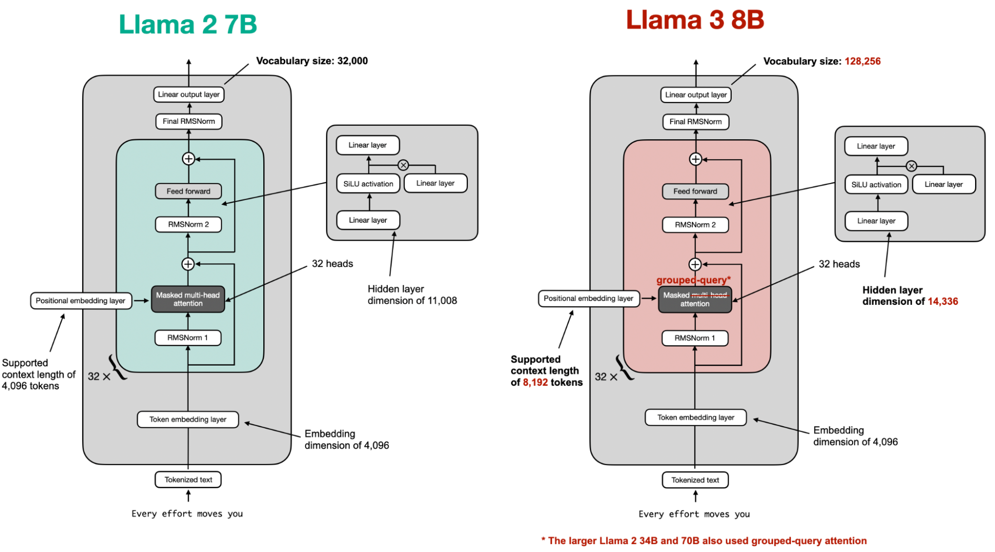
If you’re curious about architectural details, a great way to learn is by implementing the model from scratch and loading pretrained weights as a sanity check. I have a GitHub repository with a from-scratch implementation that converts GPT-2 to Llama 2, Llama 3, Llama 3.1, and Llama 3.2.

7.2 Llama 3 training

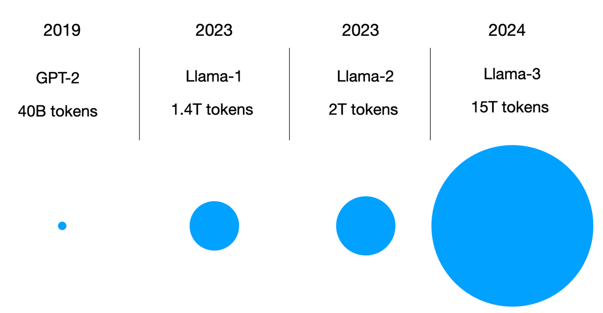
Another noteworthy update over Llama 2 is that Llama 3 has now been trained on 15 trillion tokens.

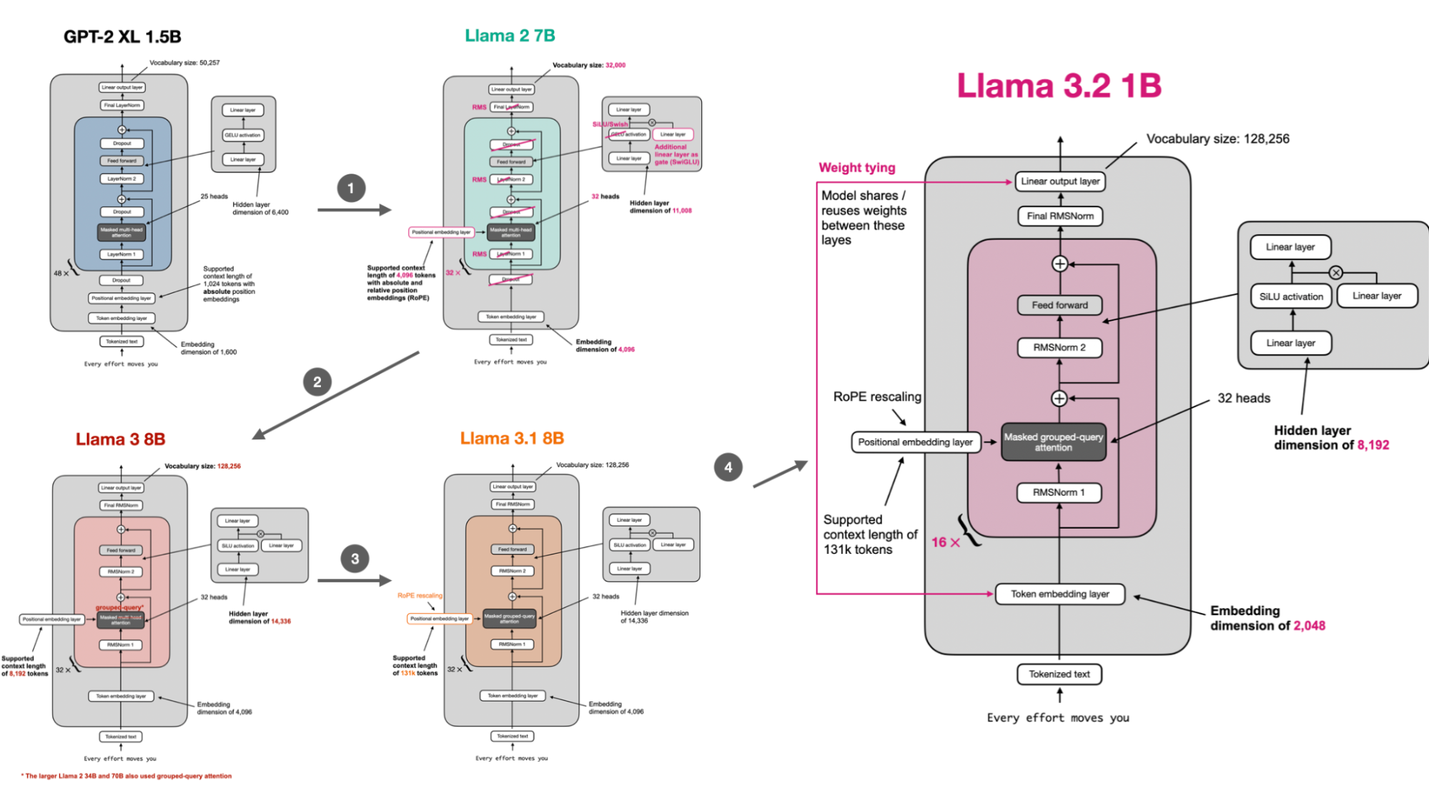
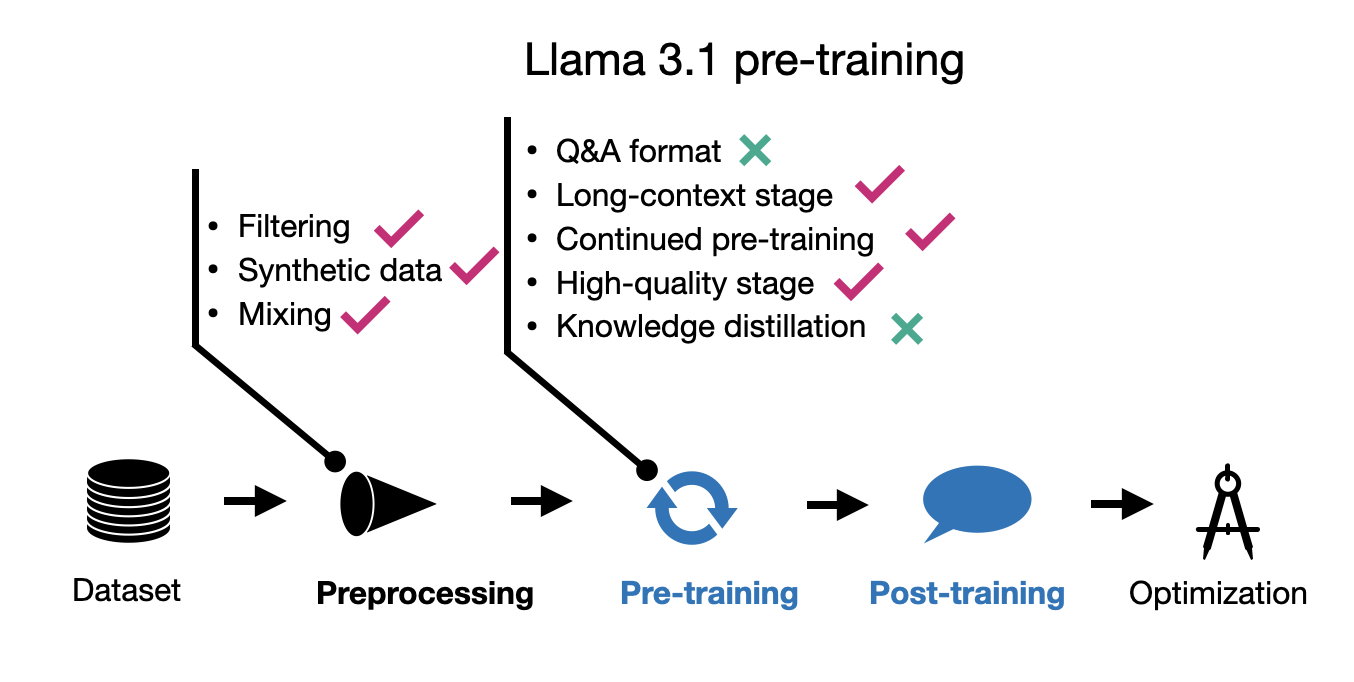
The pre-training process is now multi-staged. The paper primarily focuses on Llama 3.1, and for the sake of brevity, I have summarized its pre-training techniques in the figure below.

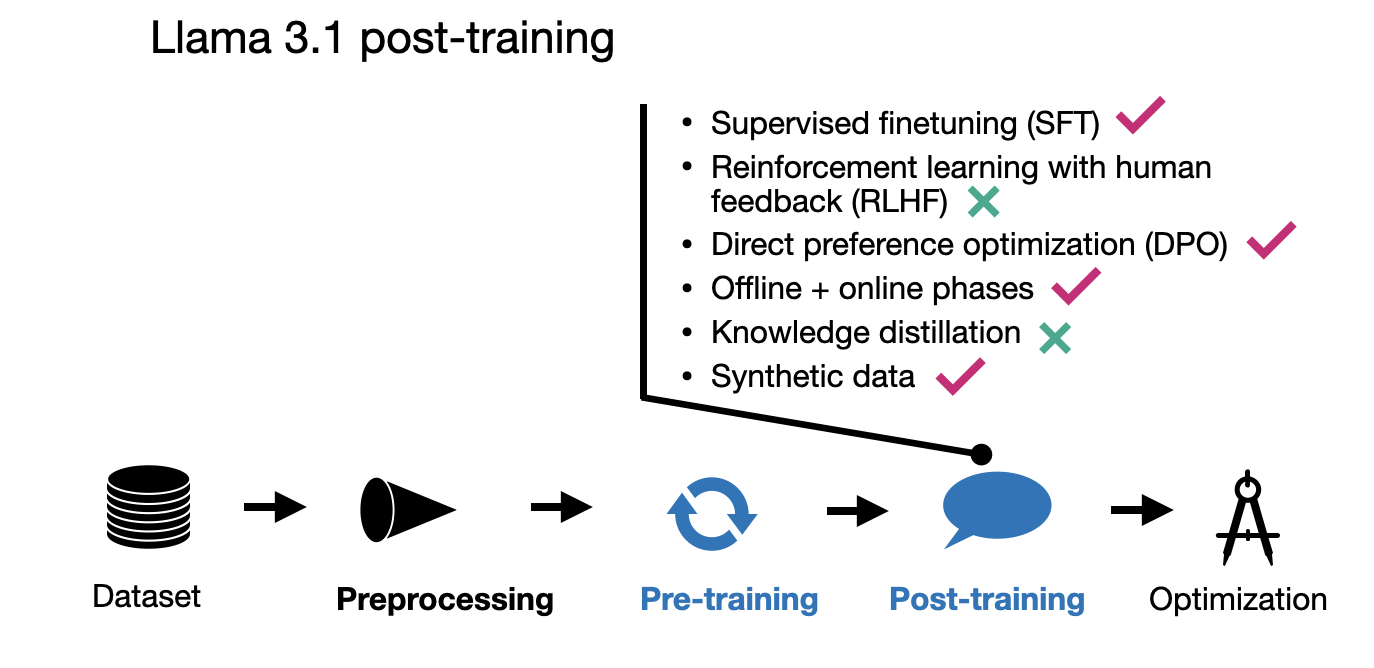
In post-training, a notable change from Llama 2 is the switch from RLHF-PPO to DPO. These methods are also summarized in the figure below.

For the interest of brevity, since there are 5 more papers to be covered in this article, I will defer the additional details and comparisons to other models to one of my previous articles. New LLM Pre-training and Post-training Paradigms.

7.3 Multimodal Llamas

Note that Llama 3.2 models were also released with multimodal support. However, I haven’t observed widespread use of these models in practice, and they aren’t widely discussed. We’ll revisit multimodal techniques in the September section later in this article.

7.4 Llama 3 impact and usage

While it’s been over half a year since Llama 3 was released, Llama models continue to be among the most widely recognized and used open-weight LLMs (based on my personal perception, as I don’t have a specific source to cite). These models are relatively easy to understand and use. The reason for their popularity is likely the Llama brand recognition coupled with robust performance across a variety of general tasks, and making it easy to finetune them.

Meta AI has also maintained momentum by iterating on the Llama 3 model, releasing versions 3.1, 3.2, and now 3.3, which span a variety of sizes to cater to diverse use cases, from on-device scenarios (1B) to high-performance applications (400B).

Although the field now includes many competitive open-source and open-weight LLMs like Olmo 2, Qwen 2.5, Gemma 2, and Phi-4, and many others, I believe Llama will remain the go-to model for most users, much like ChatGPT has retained its popularity despite competition from options like Anthropic Claude, Google Gemini, DeepSeek, and others.

Personally, I’m excited for Llama 4, which I hope will be released sometime in 2025.

8. August: Improving LLMs by scaling inference-time compute

My pick for this month is Scaling LLM Test-Time Compute Optimally can be More Effective than Scaling Model Parameters (August 2024) because it is a very well-written and detailed paper that offers some interesting insights into improving LLM responses during inference time (i.e., deployment).

8.1 Improve outputs by using more test-time computation

The main premise of this paper is to investigate if and how increased test-time computation can be used to improve LLM outputs. As a rough analogy, suppose that humans, on hard tasks, can generate better responses if they are given more time to think. Analogously, LLMs may be able to produce better outputs given more time/resources to generate their responses. In more technical terms, the researchers try to find out how much better models can perform than they are trained to do if additional compute is used during inference.

In addition, the researchers also looked into whether, given a fixed compute budget, spending more compute on test time can improve the results over spending that compute for further pre-training a model. But more on that later.

8.2 Optimizing test-time computation techniques

The paper describes techniques for increasing and improving and test-time compute in great detail, and if you are serious about deploying LLMs in practice (e.g., the aforementioned Llama models), I highly recommend giving this paper a full read.

In short, the 2 main methods to scale test-time compute are

1. Generating multiple solutions and using a process-based verifier reward model (it has to be separately trained) to select the best response

2. Updating the model’s response distribution adaptively, which essentially means revising the responses during inference generation (this also requires a separate model).

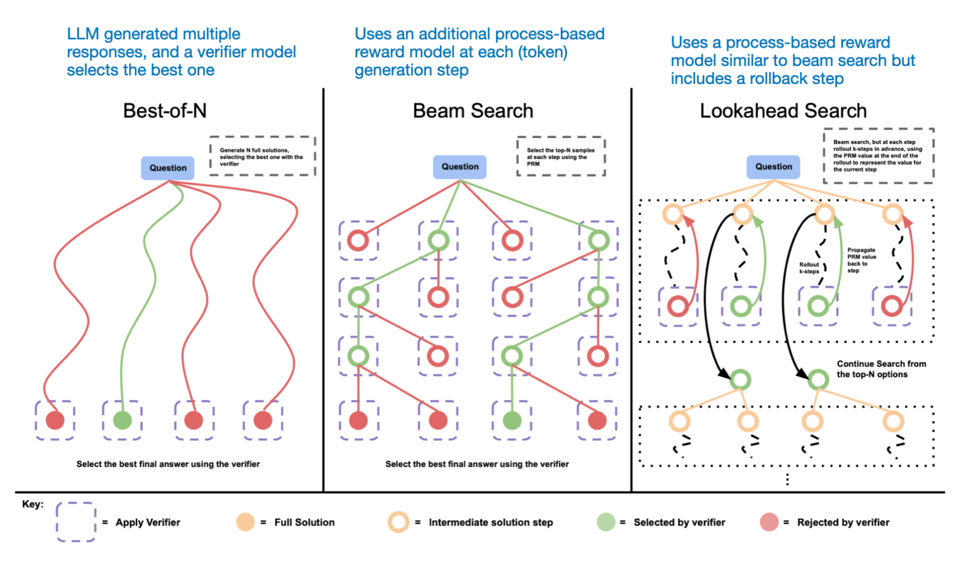
To provide a simple example for category 1: One naive way to improve test time compute is to use best-of-N sampling. This means that we let the LLM generate multiple answers in parallel and then pick the best one based on a verifier reward model. Best of N is also just one example. Multiple search algorithms fall into this category: beam-search, lookahead-search, and best-of-N, as shown in the figure below.

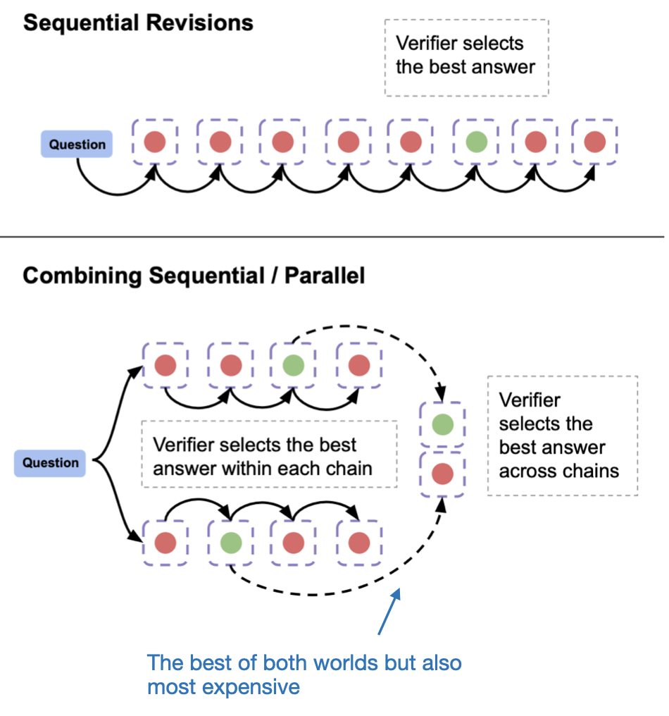
Another approach, which falls into category 2, is sequentially revising the model’s response, as illustrated in the figure below.

Which approach works better? Unfortunately, there is no one-size-fits-all answer. It depends on the base LLM and the specific problem or query. For example, revision-based approaches perform better on harder questions, and they can actually harm performance on easy questions.

In the paper, they developed an “optimal” strategy based on a model that assesses the query’s difficulty level and then chooses the right strategy appropriately.

8.3 Test-time computation versus pretraining a larger model

An interesting question to answer is, given a fixed compute budget, what gives the bigger bang for the buck: using a larger model or using an increased inference-time budget?

Here, suppose the price you pay for a query is the same because running a large model in inference is more costly than a small one.

They found that for challenging questions, larger models outperform smaller models that get additional inference compute via the inference scaling strategies discussed earlier.

However, for easy and medium questions, inference time compute can be used to match the performance of 14x larger models at the same compute budget!

8.4 Future relevance of test-time compute scaling

When using open-weight models like Llama 3 and others, we often let them generate responses as-is. However, as this paper highlights, response quality can be significantly enhanced by allocating more inference compute. (If you are deploying models, this is definitely THE paper to read.)

Of course, increasing the inference-compute budget for large, expensive models makes them even costlier to operate. Yet, when applied selectively based on the difficulty of the queries, it can provide a valuable boost in quality and accuracy for certain responses, which is something most users would undoubtedly appreciate. (It’s safe to assume that OpenAI, Anthropic, and Google already leverage such techniques behind the scenes.)

Another compelling use case is enhancing the performance of smaller, on-device LLMs. I think this will remain a hot topic in the months and years ahead as we’ve also seen with the big announcements and investments in Apple Intelligence and Microsoft’s Copilot PCs.

9. September: Comparing multimodal LLM paradigms

Multimodal LLMs were one of the major things I thought would make big leaps in 2024. And yes, we got some more open-weight LLMs this year!

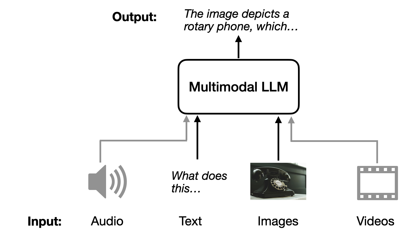
One paper that particularly stood out to me was NVIDIA’s NVLM: Open Frontier-Class Multimodal LLMs (September 2024) by Dai and colleagues, because it nicely compares the two leading multimodal paradigms.

9.1 Multimodal LLM paradigms

There are two main approaches to building multimodal LLMs:

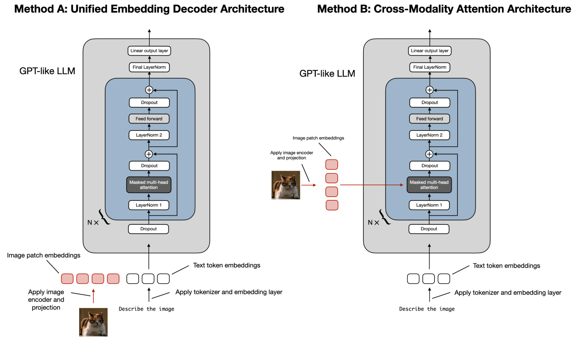
As illustrated in the figure above, the Unified Embedding-Decoder Architecture (Method A) relies on a single decoder model, resembling an unmodified LLM architecture such as GPT-2 or Llama 3.2. This method converts images into tokens that share the same embedding size as text tokens, enabling the LLM to process concatenated text and image input tokens.

In contrast, the Cross-Modality Attention Architecture (Method B) incorporates a cross-attention mechanism to integrate image and text embeddings within the attention layer directly.

If you are interested in additional details, I dedicated a whole article to multimodal LLMs earlier this year that goes over these two methods step by step: Understanding Multimodal LLMs – An introduction to the main techniques and latest models.

9.2 Nvidia’s hybrid approach

Given all the multimodal developments this year, to me, NVIDIA’s paper NVLM: Open Frontier-Class Multimodal LLMs stands out for its comprehensive apples-to-apples comparison of these multimodal approaches. Rather than focusing on a single method, they directly compared:

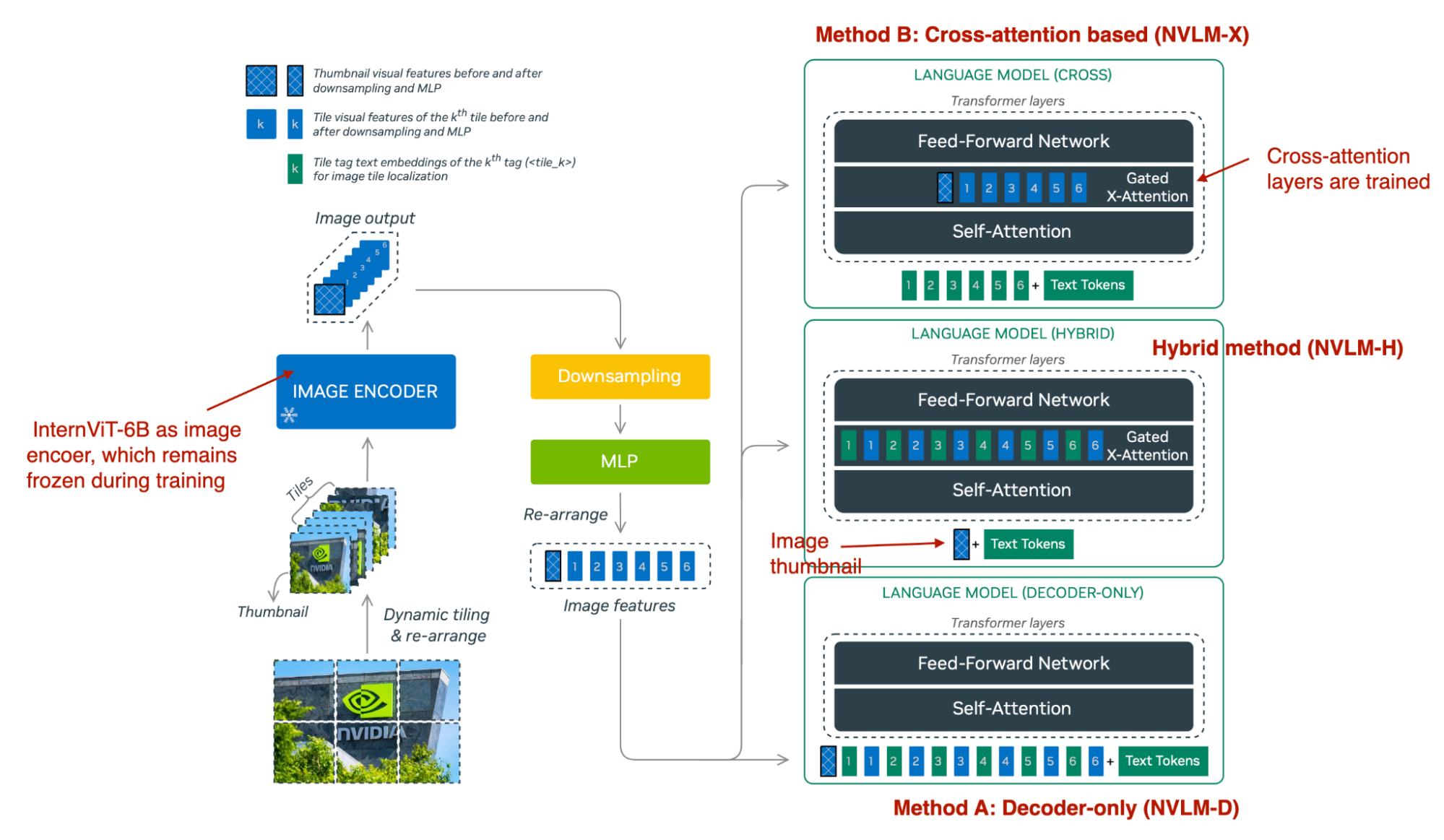
As summarized in the figure above, NVLM-D aligns with Method A, and NVLM-X corresponds to Method B, as discussed earlier. The hybrid model (NVLM-H) combines the strengths of both approaches: it first accepts an image thumbnail as input, followed by a dynamic number of patches processed through cross-attention to capture finer high-resolution details.

In summary, the key findings are as follows:

9.3 Multimodal LLMs in 2025

Multimodal LLMs are an interesting one. I think they are the next logical development up from regular text-based LLMs. Most LLM service providers like (OpenAI, Google, and Anthropic) support multimodal inputs like images. Personally, I need multimodal capabilities maybe 1% of the time (usually, it’s something like: “extract the table in markdown format” or something like that). I do expect the default of open-weight LLMs to be purely text-based because it adds less complexity. At the same time I do think we will see more options and widespread use of open-weight LLMs as the tooling and APIs evolve.

10. October: Replicating OpenAI O1’s reasoning capabilities

My pick for October is the O1 Replication Journey: A Strategic Progress Report – Part 1 (October 2024) by Quin and colleagues.

OpenAI ChatGPT’s o1 (and now o3) have gained significant popularity, as they seem to represent a paradigm shift in improving LLMs’ performance on reasoning tasks.

The exact details of OpenAI’s o1 remain undisclosed, and several papers have attempted to describe or replicate it. So, why did I choose this one? Its unusual structure and broader philosophical arguments about the state of academic research resonated with me. In other words, there was something distinctive about it that stood out and made it an interesting choice.

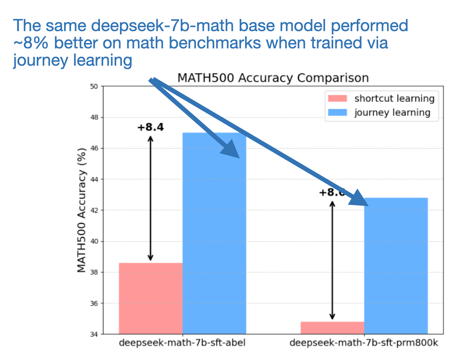
10.1 Shortcut learning vs journey learning

One of the key points of this paper is the researchers’ hypothesis that O1 employs a process called journey learning as opposed to shortcut learning, as illustrated in the figure below.

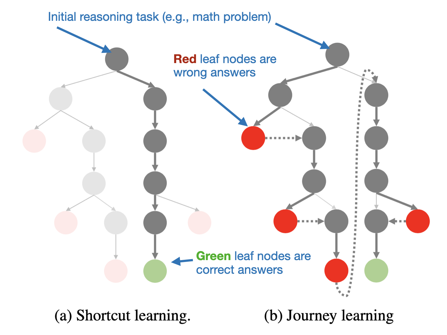
It’s worth noting that the journey learning approach is somewhat similar to the tree-based or beam-search methods with revisions, as discussed earlier in the “8. August: Improving LLMs by Scaling Inference-Time Compute” section of this article.

The subtle difference, however, is that the researchers create journey learning training examples for model finetuning, rather than simply applying this technique during inference. (It’s worth noting that I couldn’t find any information on the techniques they used to augment the inference process.)

10.2 Constructing long thoughts

The researchers constructed a reasoning tree to derive an extended thought process from it, emphasizing trial and error. This approach diverges from traditional methods that prioritize finding a direct path to the correct answer with valid intermediate steps. In their framework, each node in the reasoning tree was annotated with a rating provided by a reward model, indicating whether the step was correct or incorrect, along with reasoning to justify this evaluation.

Next, they trained a deepseek-math-7b-base model via supervised finetuning and DPO. Here, they trained two models.

1. First they used the traditional shortcut training paradigm where only the correct intermediate steps were provided.

2. Second, they trained the model with their proposed journey learning approach that included the thought process three with correct and incorrect answers, backtracking, and so forth.

(Sidenote: They only used 327 examples in each case!)

As shown in the figure below, the journey learning process outperformed shortcut learning by quite a wide margin on the MATH500 benchmark dataset.

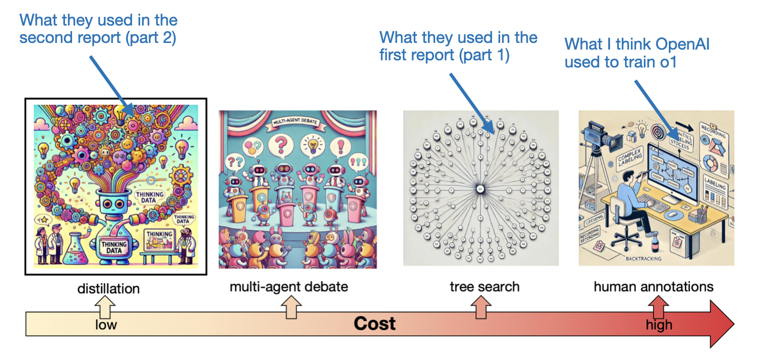
10.3 Distillation – the quick fix?

One month later, the team released another report: O1 Replication Journey – Part 2: Surpassing O1-preview through Simple Distillation, Big Progress or Bitter Lesson? (November 2024) by Huang and colleagues.

Here, they used a distillation approach, meaning they used careful prompting to extract the thought processes from o1 to train a model to reach the same performance. Since this is a long article, I won’t go over the details, but I wanted to share an interesting figure from that paper that summarizes the cost trade-offs of collecting long-thought data.

They got really good performance with this distillation approach, performing on-part with o1-preview and o1-mini. However, along with these experiments, the researchers also shared some interesting and important thoughts about the state of research in light of this approach, which I will summarize in the next section.

10.4 The state of AI research

One big focus of the part 2 report was the “Bitter Lesson of Simple Distillation”. Sure, distillation works well in practice, but it isn’t what drives progress. In the best case, using distillation, you are matching the performance of of an existing upstream model (but you are not setting a new performance record.) Below are three quotes from the paper that might serve as a warning call about the current status quo:

• “This shift from “how it works” to ‘what works’ represents a fundamental change in research mentality that could have far-reaching consequences for the field’s future innovation capacity.”
• “This erosion of first-principles thinking is particularly concerning as it undermines the very foundation of scientific innovation.”
• “Pressure to produce quick results may overshadow the value of deeper technical investigations, while students may be discouraged from pursuing more challenging, fundamental research directions.”

My personal take is that I still think there are tons of great and important ideas coming out of academic labs (today also often in partnership with industry), and they can be really practical and impactful. (A couple of my favorites that come to mind are LoRA and DPO.) The catch is that a lot of promising ideas never get tested at scale because universities usually don’t have the massive resources needed for that.

I’m not sure what the perfect solution is, and I do realize that companies can’t just give away their trade secrets. But it would be really helpful if, whenever companies do end up using ideas from academic papers, they’d openly acknowledge it. That kind of recognition goes a long way in motivating and rewarding researchers who make their work freely available. Also, it helps move the field forward by finding out what actually works in practice.

10.5 The future of LLMs in the light of o1 (and o3)

Does the O1 Replication Journey paper replicate the exact mechanism behind o1? Probably not. But it is still a valuable read full of ideas that can help achieve better results. I believe that “long-thought” models like o1 and o3 will continue to play a key role in LLM research. They are more expensive to run, but they are basically the gold standard or the upper limit for performance on reasoning tasks.

But because of their higher cost, o1-type models are not always the best option for every situation. For simpler tasks like grammar fixes or translations, we likely do not need a reasoning-heavy model. It all comes down to balancing cost and utility. We pick the right LLM for the job based on budget, latency, and other factors.

11. November: LLM scaling laws for precision

I was originally tempted to pick Allen AI’s Tulu 3: Pushing Frontiers in Open Language Model Post-Training paper because they included a detailed description of their Llama post-training methods and recipe, including ablation studies of DPO vs PPO, and a new preference alignment method called reinforcement learning with verifiable feedbacks, where they use verifiable queries where one can easily generate a ground truth answer (such as math and code questions) instead of a reward model.

But after some internal debate, I ultimately decided to go with the Scaling Laws for Precision paper (November 2024) by Kumar and colleagues, as it provides a much-needed update for the Chinchilla scaling laws from the 2022 Training Compute-Optimal Large Language Models paper that is used to determine compute-optimal LLM parameter counts and dataset sizes for pretraining.

In short, the Precision Scaling Laws paper (November 2024) extends Chinchilla’s scaling laws to account for training and inference in low-precision settings (16-bit and below), which have become very popular in recent years. For instance, this paper unifies various low-precision and quantization-related observations into a single functional form that predicts the added loss from both low-precision training and post-training quantization.

11.1 Chinchilla scaling laws refresher

The original Chinchilla scaling laws from the 2022 Training Compute-Optimal Large Language Models paper model how LLM parameter counts (N) and dataset sizes (D) jointly affect the validation loss of an LLM and are used as guidelines for deciding upon the LLM and training dataset sizes.

As a rule of thumb, the best tradeoff between dataset size D and the number of parameters N (when you have a fixed compute budget) is approximately D/N ≈ 20.

This data-parameter ratio is often referred to as “Chinchilla-optimal” because it yields lower validation loss than other ratios at the same total training cost.

Note that there are many modern exceptions, though; for example, the Llama 3 team trained on 15 trillion tokens, as discussed earlier, and for the 8B version, that’d be 15,000,000,000,000 ÷ 8,000,000,000 = 1,875, for example.

In my opinion, what’s more important than the exact data-parameter ratio is the takeaway that model and dataset sizes have to be scaled proportionally.

11.2 Low-precision training

Before discussing (or rather summarizing) the low-precision scaling laws further, let me start with a very short primer on different numeric precision formats for LLM (or deep neural network) weights in general.

To the best of my knowledge, these were the precision formats used for training GPT 2 & 3 and Llama 2 & 3 models for comparison:

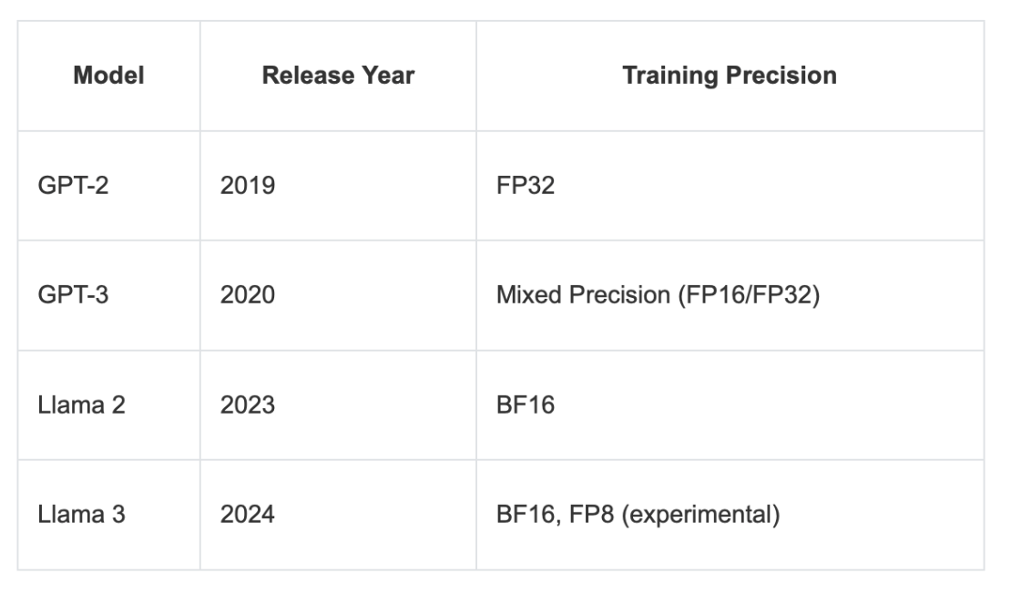
Float32 was the standard 32-bit floating-point format widely used for training deep neural networks, as it offers a good balance between range and precision. Everything below float32 is nowadays considered low-precision (although the definition of “low” is kind of a moving goalpost similar to the “large” in large language models).

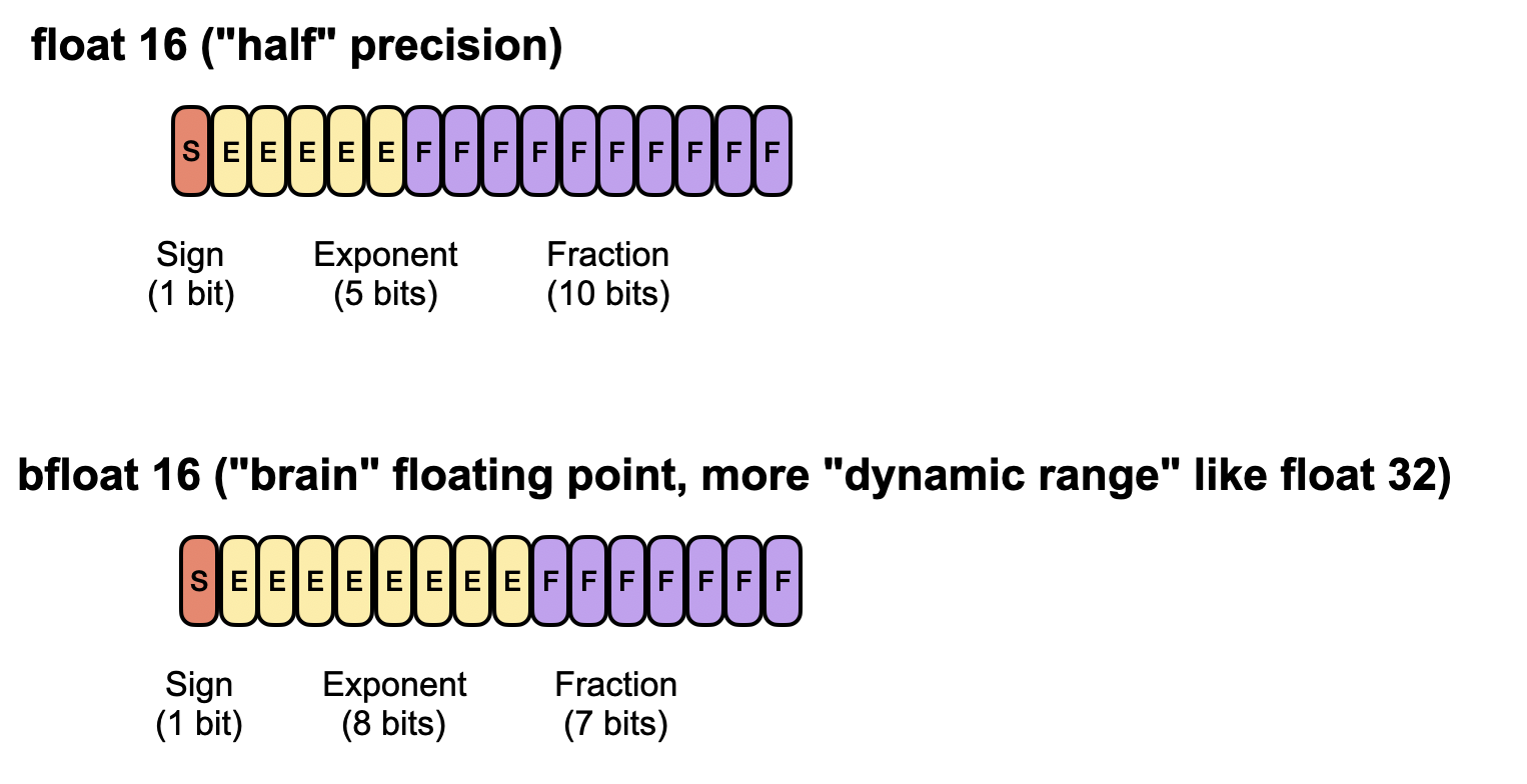
Float16, or half-precision, uses just 16 bits, saving memory and speeding up computation but providing a narrower dynamic range.

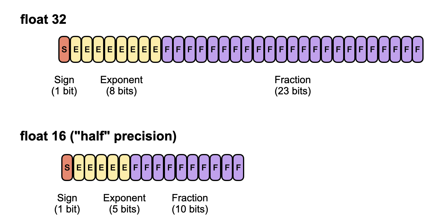
Bfloat16 (brain float 16) is also a 16-bit format but trades off some of float16’s precision for a larger exponent, allowing it to represent very large and very small numbers more effectively. As a result, bfloat16 can help avoid numeric overflow or underflow in deep learning applications, although its lower precision can still lead to rounding errors.

If you want to learn more about the different precision formats and their impact on LLM model behavior, you might like the lengthier intro in my previous The Missing Bits: Llama 2 Weights Have Changed article.

Also note that I am only showing 32- and 16-bit formats, whereas there’s currently a race to even lower precisions for training, e.g., the 8-bit format that was mentioned (as experimental) in the Llama 3 paper. (The DeepSeek-v3 model that was released on Dec 26 was entirely pretrained in 8-bit floating point precision.)

11.3 Precision scaling laws takeaways

It’s a long and interesting paper that I recommend reading in full. However, to get to the main point, the researchers extend the original Chinchilla scaling laws by adding a “precision” factor P. Concretely, they reinterpret the model parameter count N as an “effective parameter count” that shrinks as the precision decreases. (For the mathematical formulas, defer to the paper.)

Plus, they added an extra term to capture how post-training quantization degrades model performance. (I realize that I didn’t write an intro to quantization, but due to the excessive length of this article already, I may have to defer this to another time.)

The figure below is a nice illustration that more pretraining data is not always better and can actually be harmful if models are quantized after training with very small precision (int3), which I found super interesting.

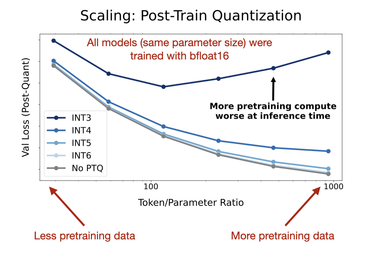
So, as a takeaway from the figure above, one might say that models trained on more and more data (like Llama 3) become harder to quantize to lower precision formats after training due to being “overtrained” on too much data.

11.4 Model scaling laws in 2025

Besides providing a much-needed update to the Chinchilla scaling laws, the research on Precision Scaling Laws provides an interesting perspective on a critical challenge for 2025: as models like LLaMA-3 are trained on larger datasets, they may become harder to quantize to low precision formats like INT3 without performance loss.

This finding underscores the need to rethink the “more data is better” mindset, balancing dataset size with the practical constraints of efficient inference. It’s also an important insight for driving hardware optimization.

One of the aspects that I think is often neglected in these scaling laws studies is the dataset’s quality. I think the pretraining data’s nature can have a significant impact. (More on that in the Phi-4 discussion below.)

12. December: Phi-4 and learning from synthetic data

Several interesting models were released in the latter half of 2024, including the impressive DeepSeek-V3 on Christmas day. While it might not be the biggest model release, ultimately, I decided to go with Microsoft’s Phi-4 Technical Report because it offers interesting insights into the use of synthetic data.

12.1 Phi-4 performance

The Phi-4 Technical Report (December 2024) by Abdin and colleagues describes the training of Microsoft’s latest 14-billion-parameter open-weight LLM. What makes Phi-4 particularly interesting is that it was trained primarily on synthetic data generated by GPT-4o. According to the benchmarks, it outperforms other LLMs of a similar size, including its predecessor, Phi-3, which was trained predominantly on non-synthetic data.

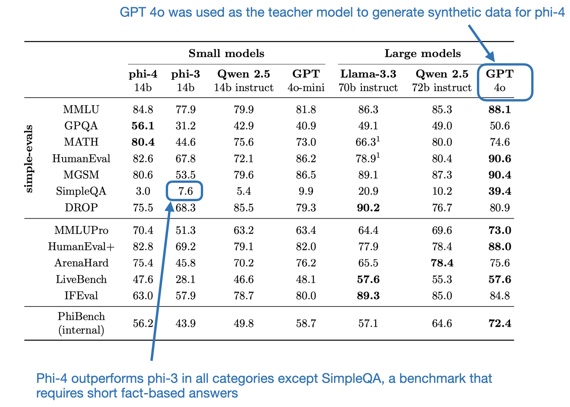
I’m not entirely sure why the model performs worse on SimpleQA, as shown in the table above. But one possible explanation is that SimpleQA is a relatively new benchmark, released on October 30, 2024. Since it was developed by OpenAI as part of their evaluation suite, it might not have been included in the training data for GPT-4o or incorporated into the web-crawled datasets. Furthermore, because GPT-4o was used to generate the synthetic data for this evaluation, none of the models would have encountered SimpleQA during training. However, phi-4 might be overfitting to other benchmarks, which could explain its comparatively lower performance on this unseen SimpleQA dataset. Anyways, that’s just my hypothesis.

12.2 Synthetic data learnings

Let’s look at the dataset composition before summarizing some of the ablation studies presented in this paper.

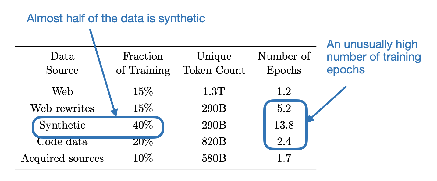
The researchers observed that while synthetic data is generally beneficial, models trained exclusively on synthetic data performed poorly on knowledge-based benchmarks. To me, this raises the question: does synthetic data lack sufficient knowledge-specific information, or does it include a higher proportion of factual errors, such as those caused by hallucinations?

At the same time, the researchers found that increasing the number of training epochs on synthetic data boosted the performance more than just adding more web data, as shown in the figure below.

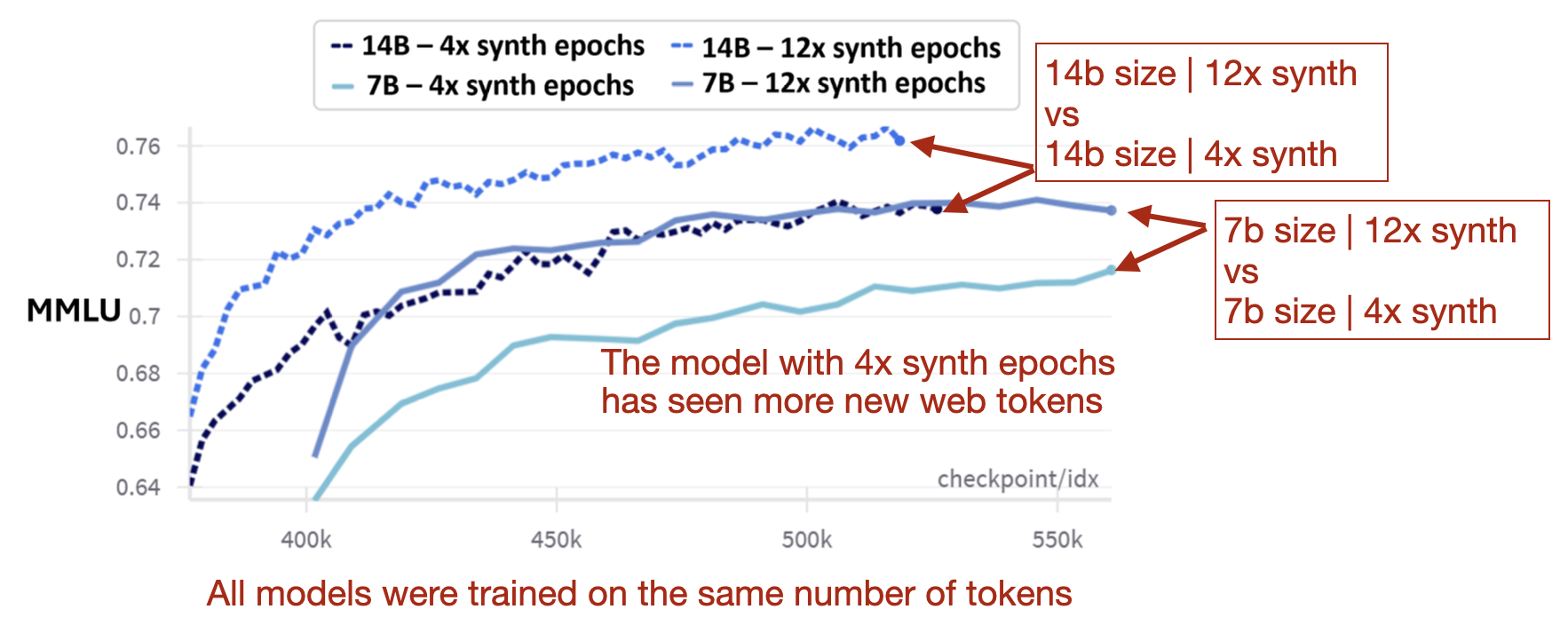
In summary, an excessive proportion of synthetic data in the mix negatively impacts knowledge-based performance. However, within a more balanced synthetic-to-web data mix, increasing the number of iterations (epochs) over the synthetic dataset is beneficial.

12.4 Future importance of synthetic data

The phi-4 technical report offers interesting insights into the use of synthetic data, namely that it can be highly beneficial for model pre-training. Especially since scaling laws are said to be plateauing concerning both model and dataset sizes (although the Llama 3 paper noted that they haven’t seen a convergence at the 15T token level yet), researchers and engineers are looking for alternative ways to keep pushing the envelope. Of course, the refinement and addition of pre- and especially post-training techniques will likely remain one of the big needle movers. Still, I think that the use of synthetic data will be regarded as an effective way to either create a) pretrained base models with less data or b) create even better base models (think 15 trillion tokens from the Llama 3 dataset plus 40% synthetic data tokens added to it).

I see the use of high-quality data as analogous to transfer learning. Instead of pre-training a model on raw, unstructured internet data and refining it during post-training, leveraging (some) synthetic data generated by a high-quality model (such as GPT-4o, which has already undergone extensive refinement) may serve as a kind of jumpstart. In other words, the use of high-quality training data might enable the model to learn more effectively from the outset.

Conclusions and outlook

I hope you found these research summaries useful! As always, this article ended up being longer than I originally intended. But let me close out with a relatively short and snappy section on my predictions (or expectations) for 2025.

Multimodal LLMs

Last year, I predicted LLMs would become increasingly multimodal. Now, all major proprietary LLM providers offer multimodal (or at least image) support. So, the transformation is now fully underway, and we will also see more open-source efforts toward this.

Based on what I’ve seen and read, there’s definitely been a sharp increase in multimodal papers. Maybe followed by my open-source finetuning methods and resources; although I’d argue for many use cases, text-only suffices and will continue to suffice, and the main focus will be on developing better reasoning models (like o1 and the upcoming o3).

Computational efficiency

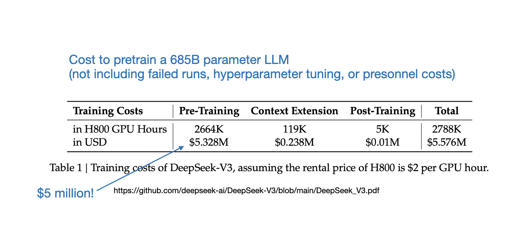
Pretraining and using LLMs is relatively expensive. So, I expect that we are going to see more clever tricks to improve computational efficiency of LLMs in the foreseeable future. For reference, training the recent DeepSeek-v3 model would cost $5 million dollars assuming the GPU rental sticker prices (and this doesn’t include hyperparameter tuning, failed runs, and personnel cost).

By the way, according to the official Meta AI Llama 3 model card, Llama 3 405B used even ~10x more compute (30.84 million GPU hours vs 2.66 million GPU hours).

Popular examples of techniques to make LLMs efficient (although not all apply during training) include a mixture of experts (as discussed in my part 1 article), grouped-query attention as found in Llama models, and many others. Another interesting one is the use of multihead latent attention, as found in DeepSeek models, to make KV-caching in multihead attention more efficient.

Another interesting recent route is targeting the model input. For instance, the recently proposed Byte Latent Transformer improves efficiency by dynamically encoding bytes into entropy-based patches, optimizing compute for scalability and faster inference without tokenization.

State space models

You may have noticed that I didn’t cover state space models this year. That’s because my current focus is primarily on transformer-based LLMs. While I find state space models super interesting, they still seem quite experimental at this stage. Besides, transformers continue to demonstrate exceptional performance across a wide range of tasks, making it not very tempting to consider alternatives.

However, that doesn’t mean there hasn’t been any progress on the state space model front. I’ve seen a bunch of interesting papers in this area. And one interesting trend I noticed is that they are now all more or less hybrid models integrating self-attention from transformer models. For example,

• Jamba-1.5: Hybrid Transformer-Mamba Models at Scale,
• The Mamba in the Llama: Distilling and Accelerating Hybrid Models,
• and Samba: Simple Hybrid State Space Models for Efficient Unlimited Context Language Modeling.

In that sense, they are also getting more computationally expensive. With efficiency tweaks to transformer-based LLMs and adding attention to state space models, they will probably meet somewhere in the middle if the current trends continue.  It’s definitely an interesting field of research to watch though.

Scaling

Towards the end of the year, there was also some discussion of LLM scaling “being over” as there is no more internet data. This discussion came from a NeurIPS talk by Ilya Sutskever (one of OpenAI’s co-founders and co-author on the GPT papers), but unfortunately, I couldn’t attend the conference this year, so I am not familiar with the details.

In any case, it’s an interesting point because the internet grows exponentially fast. I could find resources saying that it grows ”15.87 terabytes of data daily.” Sure, the challenge is that not all of the data is text or useful for LLM training. However, as we have seen with Phi-4, there are still a lot of opportunities in data curation and refinement that can help make some leaps from training data alone.

I agree with the diminishing returns of scaling via data, though. I expect that the gains will be smaller as we are probably heading towards plateauing. It’s not a bad thing, though, as it brings other improvement opportunities.

One notable area where I expect a lot of future gains to come from is post-training. We’ve already seen a taste of these developments in this area with recent LLM releases, as I wrote about last summer in my New LLM Pre-training and Post-training Paradigms article.

What I am looking forward to

I really enjoyed tinkering and (re)implementing the various Llama models (3, 3.1, and 3.2) this year. I am really looking forward to the Llama 4 release, which hopefully also comes in small and convenient sizes that I can experiment with on my laptop or affordable cloud GPUs.

Moreover, it’s also the year where I want to experiment more with special-purpose model finetuning rather than generating general chatbots (it’s already pretty crowded in this space). We’ve seen a bit of that with various code and math models (the recent Qwen 2.5 Coder and Qwen 2.5 Math come to mind, which I unfortunately haven’t had a chance to cover in this report yet).

In any case, I could keep on going with this wish list and plans, as 2025 will be another interesting and fast-moving year! It’s definitely not going to be boring, that’s for sure!