Understanding and Coding the KV Cache in LLMs from Scratch
KV caches are one of the most critical techniques for efficient inference in LLMs in production. KV caches are an important component for compute-efficient LLM inference in production. This article explains how they work conceptually and in code with a from-scratch, human-readable implementation.
It’s been a while since I shared a technical tutorial explaining fundamental LLM concepts. As I am currently recovering from an injury and working on a bigger LLM research-focused article, I thought I’d share a tutorial article on a topic several readers asked me about (as it was not included in my Building a Large Language Model From Scratch book).
Happy reading!
Overview
In short, a KV cache stores intermediate key (K) and value (V) computations for reuse during inference (after training), which results in a substantial speed-up when generating text. The downside of a KV cache is that it adds more complexity to the code, increases memory requirements (the main reason I initially didn’t include it in the book), and can’t be used during training. However, the inference speed-ups are often well worth the trade-offs in code complexity and memory when using LLMs in production.
What Is a KV Cache?
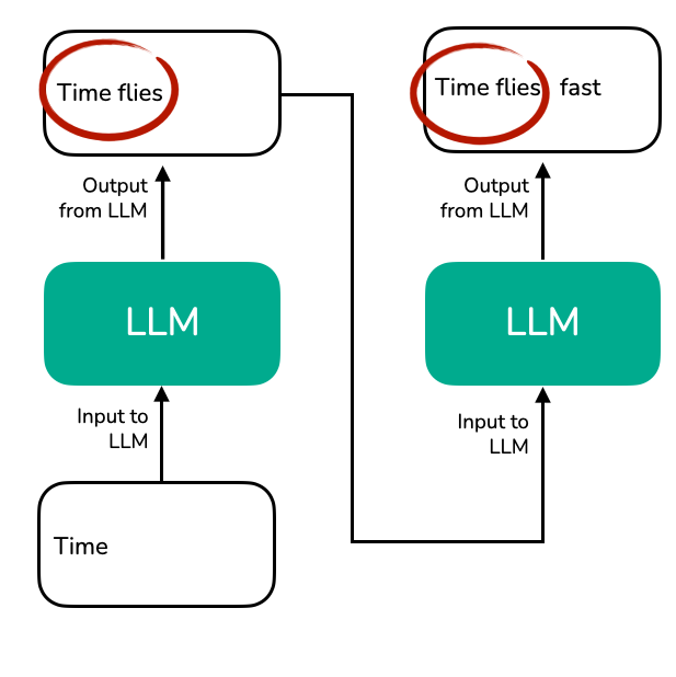
Imagine the LLM is generating some text. Concretely, suppose the LLM is given the following prompt: “Time”. As you may already know, LLMs generate one word (or token) at a time, and the two following text generation steps may look as illustrated in the figure below:

Note that there is some redundancy in the generated LLM text outputs, as highlighted in the next figure:
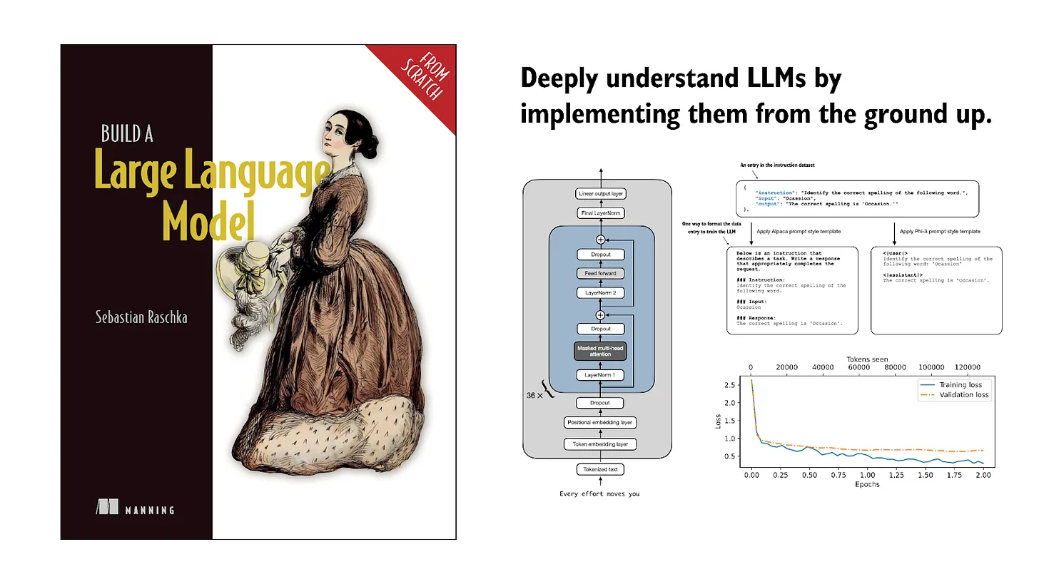
When we implement an LLM text generation function, we typically only use the last generated token from each step. However, the visualization above highlights one of the main inefficiencies on a conceptual level. This inefficiency (or redundancy) becomes more clear if we zoom in on the attention mechanism itself. (If you are curious about attention mechanisms, you can read more in Chapter 3 of my Build a Large Language Model (From Scratch) book or my Understanding and Coding Self-Attention, Multi-Head Attention, Causal-Attention, and Cross-Attention in LLMs article).
The following figure shows an excerpt of an attention mechanism computation that is at the core of an LLM. Here, the input tokens (“Time” and “flies”) are encoded as 3-dimensional vectors (in reality, these vectors are much larger, but this would make it challenging to fit them into a small figure). The matrices W are the weight matrices of the attention mechanism that transform these inputs into key, value, and query vectors.
The figure below shows an excerpt of the underlying attention score computation with the key and value vectors highlighted:

k) and value (v) vectors from token embeddings during attention computation. Each input token (e.g., "Time" and "flies") is projected using learned matrices W\_k and W\_v to obtain its corresponding key and value vectors.As mentioned earlier, LLMs generate one word (or token) at a time. Suppose the LLM generated the word “fast” so that the prompt for the next round becomes “Time flies fast”. This is illustrated in the next figure below:
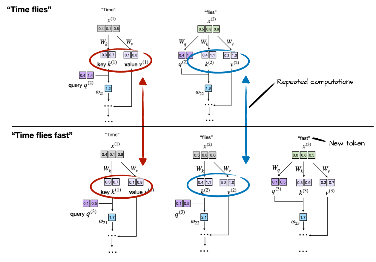
k(1)/v(1) and k(2)/v(2) vectors again, rather than reusing them. This repeated computation highlights the inefficiency of not using a KV cache during autoregressive decoding.As we can see, based on comparing the previous 2 figures, the keys and value vectors for the first two tokens are exactly the same, and it would be wasteful to recompute them in each next-token text generation round.
Now, the idea of the KV cache is to implement a caching mechanism that stores the previously generated key and value vectors for reuse, which helps us to avoid these unnecessary recomputations.
How LLMs Generate Text (Without and With a KV Cache)
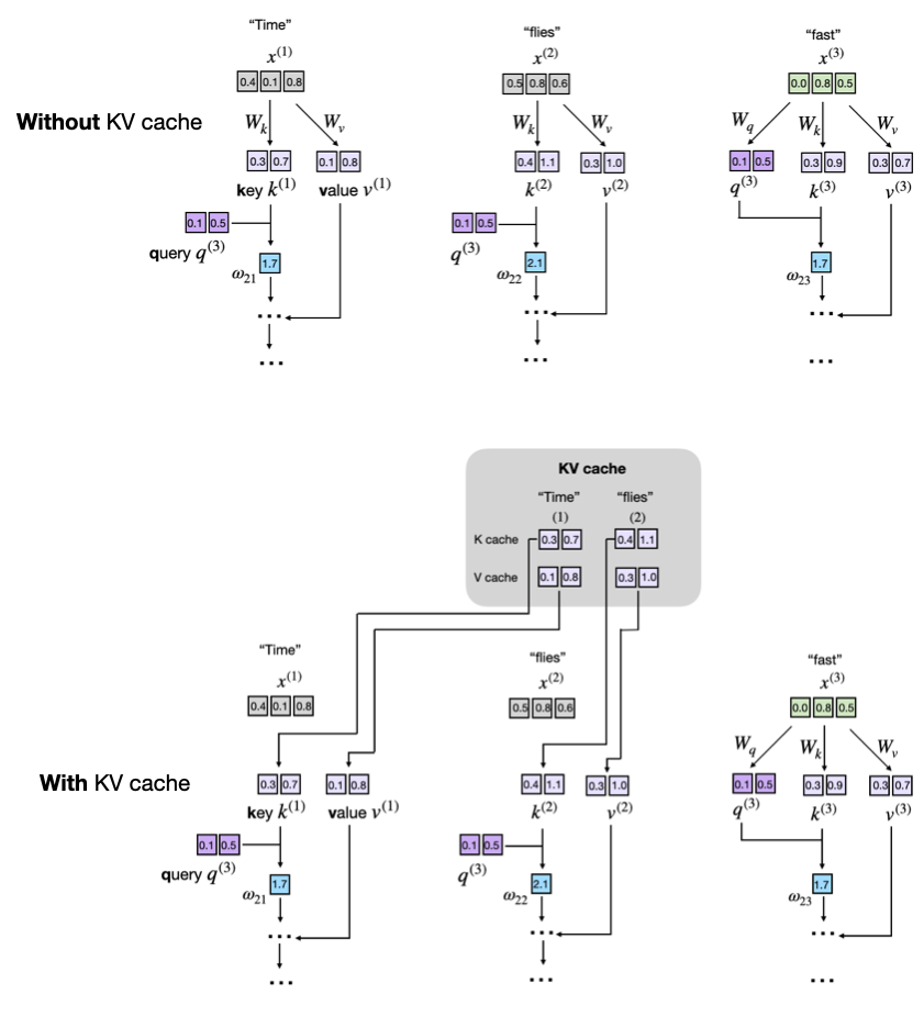
After we went over the basic concept in the previous section, let’s go into a bit more detail before we look at a concrete code implementation. If we have a text generation process without KV cache for “Time flies fast”, we can think of it as follows:
Notice the redundancy: tokens “Time” and “flies” are recomputed at every new generation step. The KV cache resolves this inefficiency by storing and reusing previously computed key and value vectors:
- Initially, the model computes and caches key and value vectors for the input tokens.
- For each new token generated, the model only computes key and value vectors for that specific token.
- Previously computed vectors are retrieved from the cache to avoid redundant computations.
The table below summarizes the computation and caching steps and states:
The benefits here are that "Time" is computed once and reused twice, and "flies" is computed once and reused once. (It’s a short text example for simplicity, but it should be intuitive to see that the longer the text, the more we get to reuse already computed keys and values, which increases the generation speed.)n speed.)
The following figure illustrates generation step 3 with and without a KV cache side by side.
So, if we want to implement a KV cache in code, all we have to do is compute the keys and values as usual but then store them so that we can retrieve them in the next round. The next section illustrates this with a concrete code example.
Implementing a KV Cache from Scratch
There are many ways to implement a KV cache, with the main idea being that we only compute the key and value tensors for the newly generated tokens in each generation step.
I opted for a simple one that emphasizes code readability. I think it’s easiest to just scroll through the code changes to see how it’s implemented.
There are two files I shared on GitHub, which are self-contained Python scripts that implement an LLM with and without KV cache from scratch:
gpt_ch04.py: Self-contained code taken from Chapters 3 and 4 of my Build a Large Language Model (From Scratch) book to implement the LLM and run the simple text generation functiongpt_with_kv_cache.py: The same as above, but with the necessary changes made to implement the KV cache.
To read through the KV cache-relevant code modifications, you can either:
a. Open the gpt_with_kv_cache.py file and look out for the # NEW sections that mark the new changes:
b. Check out the two code files via a file diff tool of your choice to compare the changes:
In additoin, to summarize the implementation details, there’s a short walkthrough in the following subsections.
1. Registering the Cache Buffers
Inside the MultiHeadAttention constructor, we add two non-persistent buffers, cache_k and cache_v, which will hold concatenated keys and values across steps:
self.register_buffer("cache_k", None, persistent=False)
self.register_buffer("cache_v", None, persistent=False)
(I made a YouTube video if you want to learn more about buffers: Understanding PyTorch Buffers.)
2. Forward pass with use_cache flag
Next, we extend the forward method of the MultiHeadAttention class to accept a use_cache argument:
def forward(self, x, use_cache=False):
    b, num_tokens, d_in = x.shape

    keys_new = self.W_key(x)  # Shape: (b, num_tokens, d_out)
    values_new = self.W_value(x)
    queries = self.W_query(x)
    #...

    if use_cache:
        if self.cache_k is None:
            self.cache_k, self.cache_v = keys_new, values_new
        else:
            self.cache_k = torch.cat([self.cache_k, keys_new], dim=1)
            self.cache_v = torch.cat([self.cache_v, values_new], dim=1)
        keys, values = self.cache_k, self.cache_v
    else:
        keys, values = keys_new, values_new
The storage and retrieval of keys and values here implements the core idea of the KV cache.
Storing
Concretely, after the cache is initialized via the if self.cache_k is None: ..., we add the newly generated keys and values via self.cache_k = torch.cat(...) and self.cache_v = torch.cat(...) to the cache, respectively.
Retrieving
Then, keys, values = self.cache_k, self.cache_v retrieves the stored values and keys from the cache.
And that’s basically it: the core store & retrieve mechanism of a KV cache. The following sections, 3 and 4, just take care of minor implementation details.
3. Clearing the Cache
When generating text, we have to remember to reset both the keys and value buffers between two separate text-generation calls. Otherwise, the queries of a new prompt will attend to stale keys left over from the previous sequence, which causes the model to rely on irrelevant context and produce incoherent output. To prevent this, we add a reset_kv_cache method to the MultiHeadAttention class that we can use between text-generation calls later:
def reset_cache(self):
    self.cache_k, self.cache_v = None, None
4. Propagating use_cache in the Full Model
With the changes to the MultiHeadAttention class in place, we now modify the GPTModel class. First, we add a position tracking for the token indices to the instructor:
self.current_pos = 0
This is a simple counter that remembers how many tokens the model has already cached during an incremental generation session.
Then, we replace the one-liner block call with an explicit loop, passing use_cache through each transformer block:
def forward(self, in_idx, use_cache=False):
    # ...

    if use_cache:
        pos_ids = torch.arange(
            self.current_pos, self.current_pos + seq_len,
            device=in_idx.device, dtype=torch.long
        )
        self.current_pos += seq_len
    else:
        pos_ids = torch.arange(
            0, seq_len, device=in_idx.device, dtype=torch.long
        )

    pos_embeds = self.pos_emb(pos_ids).unsqueeze(0)
    x = tok_embeds + pos_embeds
    # ...
    for blk in self.trf_blocks:
        x = blk(x, use_cache=use_cache)
What happens above if we set use_cache=True is that we start at the self.current_pos and count seq_len steps. Then, bump the counter so the next decoding call continues where we left off.
The reason for the self.current_pos tracking is that new queries must line up directly after the keys and values that are already stored. Without using a counter, every new step would start at position 0 again, so the model would treat the new tokens as if they overlapped the earlier ones. (Alternatively, we could also keep track via an offset = block.att.cache_k.shape[1].)
The above change then also requires a small modification to the TransformerBlock class to accept the use_cache argument:
def forward(self, x, use_cache=False):
    # ...
    self.att(x, use_cache=use_cache)
Lastly, we add a model-level reset to GPTModel to clear all block caches at once for our convenience:
def reset_kv_cache(self):
    for blk in self.trf_blocks:
        blk.att.reset_cache()
    self.current_pos = 0
5. Using the Cache in Generation
With the changes to the GPTModel, TransformerBlock, and MultiHeadAttention, finally, here’s how we use the KV cache in a simple text generation function:
def generate_text_simple_cached(
        model, idx, max_new_tokens, use_cache=True
    ):
    model.eval()

    ctx_len = model.pos_emb.num_embeddings  # max sup. len., e.g. 1024
    if use_cache:
        # Init cache with full prompt
        model.reset_kv_cache()
        with torch.no_grad():
            logits = model(idx[:, -ctx_len:], use_cache=True)

        for _ in range(max_new_tokens):
            # a) pick the token with the highest log-probability
            next_idx = logits[:, -1].argmax(dim=-1, keepdim=True)
            # b) append it to the running sequence
            idx = torch.cat([idx, next_idx], dim=1)
            # c) feed model only the new token
            with torch.no_grad():
                logits = model(next_idx, use_cache=True)
    else:
        for _ in range(max_new_tokens):
            with torch.no_grad():
                logits = model(idx[:, -ctx_len:], use_cache=False)
            next_idx = logits[:, -1].argmax(dim=-1, keepdim=True)
            idx = torch.cat([idx, next_idx], dim=1)

    return idx
Note that we only feed the model the new token in c) via logits = model(next_idx, use_cache=True). Without caching, we feed the model the whole input logits = model(idx[:, -ctx_len:], use_cache=False) as it has no stored keys and values to reuse.
A Simple Performance Comparison
After covering the KV cache on a conceptual level, the big question is how well it actually performs in practice on a small example. To give the implementation a try, we can run the two aforementioned code files as Python scripts, which will run the small 124 M parameter LLM to generate 200 new tokens (given a 4-token prompt “Hello, I am” to start with):
pip install -r https://raw.githubusercontent.com/rasbt/LLMs-from-scratch/refs/heads/main/requirements.txt

python gpt_ch04.py

python gpt_with_kv_cache.py
On a Mac Mini with M4 chip (CPU), the results are as follows:
So, as we can see, we already get a ~5x speed-up with a small 124 M parameter model and a short 200-token sequence length. (Note that this implementation is optimized for code readability and not optimized for CUDA or MPS runtime speed, which would require pre-allocating tensors instead of reinstating and concatenating them.)
Note: The model generates “gibberish” in both cases, i.e., text that looks like this:
Output text: Hello, I am Featureiman Byeswickattribute argue logger Normandy Compton analogous bore ITVEGIN ministriesysics Kle functional recountrictionchangingVirgin embarrassedgl …
This is because we haven’t trained the model yet. The next chapter trains the model, and you can use the KV cache on the trained model (however, the KV cache is only meant to be used during inference) to generate coherent text. Here, we are using the untrained model to keep the code simple(r).
What’s more important, though, is that both the gpt_ch04.py and gpt_with_kv_cache.py implementations produce exactly the same text. This tells us that the KV cache is implemented correctly – it is easy to make indexing mistakes that can lead to divergent results.
Thanks for reading Ahead of AI! Subscribe for free to receive new posts and support my work.
Subscribe
KV cache Advantages and Disadvantages
As sequence length increases, the benefits and downsides of a KV cache become more pronounced in the following ways:
- [Good] Computational efficiency increases: Without caching, the attention at step t must compare the new query with t previous keys, so the cumulative work scales quadratically, O(n²). With a cache, each key and value is computed once and then reused, reducing the total per-step complexity to linear, O(n).
- [Bad] Memory usage increases linearly: Each new token appends to the KV cache. For long sequences and larger LLMs, the cumulative KV cache grows larger, which can consume a significant or even prohibitive amount of (GPU) memory. As a workaround, we can truncate the KV cache, but this adds even more complexity (but again, it may well be worth it when deploying LLMs.)
Optimizing the KV Cache Implementation
While my conceptual implementation of a KV cache above helps with clarity and is mainly geared towards code readability and educational purposes, deploying it in real-world scenarios (especially with larger models and longer sequence lengths) requires more careful optimization.
Common Pitfalls When Scaling the Cache
- Memory fragmentation and repeated allocations: Continuously concatenating tensors via
torch.cat, as shown earlier, leads to performance bottlenecks due to frequent memory allocation and reallocation. - Linear growth in memory usage: Without proper handling, the KV cache size becomes impractical for very long sequences.
Tip 1: Pre-allocate Memory
Rather than concatenating tensors repeatedly, we could pre-allocate a sufficiently large tensor based on the expected maximum sequence length. This ensures consistent memory use and reduces overhead. In pseudo-code, this may look like as follows:
# Example pre-allocation for keys and values
max_seq_len = 1024  # maximum expected sequence length
cache_k = torch.zeros(
    (batch_size, num_heads, max_seq_len, head_dim), device=device
)
cache_v = torch.zeros(
    (batch_size, num_heads, max_seq_len, head_dim), device=device
)
During inference, we can then simply write into slices of these pre-allocated tensors.
Tip 2: Truncate Cache via Sliding Window
To avoid blowing up our GPU memory, we can implement a sliding window approach with dynamic truncation. Via the sliding window, we maintain only the last window_size tokens in the cache:
# Sliding window cache implementation
window_size = 512
cache_k = cache_k[:, :, -window_size:, :]
cache_v = cache_v[:, :, -window_size:, :]
Optimizations in Practice
You can find these optimizations in the gpt_with_kv_cache_optimized.py file.
On a Mac Mini with an M4 chip (CPU), with a 200-token generation and a window size equal to the LLM’s context length (to guarantee the same results and thus a fair comparison) below, the code runtimes compare as follows:
Unfortunately, the speed advantages disappear on CUDA devices as this is a tiny model, and the device transfer and communication outweigh the benefits of a KV cache for this small model.
Conclusion
Although caching introduces additional complexity and memory considerations, the noticeable gains in efficiency typically outweigh these trade-offs, especially in production environments.
Remember, while I prioritized code clarity and readability over efficiency here, the takeaway is that practical implementations often require thoughtful optimizations, such as pre-allocating memory or applying a sliding-window cache to manage memory growth effectively. In that sense, I hope this article turned out to be informative.
Feel free to experiment with these techniques, and happy coding!
If you read the book and have a few minutes to spare, I'd really appreciate a brief review. It helps us authors a lot!
Your support means a great deal! Thank you!