Using and Finetuning Pretrained Transformers

This week has been filled with developments, including exciting new AI research that I’ll be discussing in my usual end-of-month write-ups.

Additionally, I am excited to announce the release of my new book, Machine Learning Q and AI, published by No Starch Press.

If you’ve been searching for a resource following an introductory machine learning course, this might be the one. I’m covering 30 concepts that were slightly out of scope for the previous books and courses I’ve taught, and I’ve compiled them here in a concise question-and-answer format (including exercises).

I believe it will also serve as a useful companion for preparing for machine learning interviews.

Since the different ways to use and finetune pretrained large language models are currently one of the most frequently discussed topics, I wanted to share an excerpt from the book, in hope that it might be useful for your current projects.

Happy reading!

What are the different ways to use and finetune pretrained large language models?

What are the different ways to use and finetune pretrained large language models (LLMs)? The three most common ways to use and finetune pretrained LLMs include a feature-based approach, in-context prompting, and updating a subset of the model parameters.

First, most pretrained LLMs or language transformers can be utilized without the need for further finetuning. For instance, we can employ a feature-based method to train a new downstream model, such as a linear classifier, using embeddings generated by a pretrained transformer. Second, we can showcase examples of a new task within the input itself, which means we can directly exhibit the expected outcomes without requiring any updates or learning from the model. This concept is also known as prompting. Finally, it’s also possible to finetune all or just a small number of parameters to achieve the desired outcomes.

The following sections discuss these types of approaches in greater depth.

Using Transformers for Classification Tasks

Let’s start with the conventional methods for utilizing pretrained transformers: training another model on feature embeddings, finetuning output layers, and finetuning all layers. We’ll discuss these in the context of classification. (We will revisit prompting later in the section “In-Context Learning, Indexing, and Prompt Tuning”.)

The feature-based approach

In the feature-based approach, we load the pretrained model and keep it “frozen,” meaning we do not update any parameters of the pretrained model. Instead, we treat the model as a feature extractor that we apply to our new dataset. We then train a downstream model on these embeddings. This downstream model can be any model we like (random forests, XGBoost, and so on), but linear classifiers typically perform best. This is likely because pretrained transformers like BERT, GPT, Llama, Mistral, and so on already extract high-quality, informative features from the input data. These feature embeddings often capture complex relationships and patterns, making it easy for a linear classifier to effectively separate the data into different classes.

Furthermore, linear classifiers, such as logistic regression models and support vector machines, tend to have strong regularization properties. These regularization properties help prevent overfitting when working with high-dimensional feature spaces generated by pretrained transformers. This feature-based approach is the most efficient method since it doesn’t require updating the transformer model at all. Finally, the embeddings can be precomputed for a given training dataset (since they don’t change) when training a classifier for multiple training epochs.

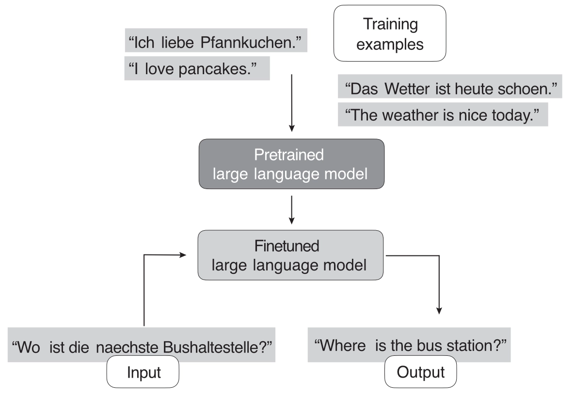
Figure 1 illustrates how LLMs are typically created and adopted for downstream tasks using finetuning. Here, a pretrained model, trained on a general text corpus, is finetuned to perform tasks like German-to-English translation.

Finetuning

The conventional methods for finetuning pretrained LLMs include updating only the output layers, a method we’ll refer to as finetuning I, and updating all layers, which we’ll call finetuning II.

Finetuning I is similar to the feature-based approach described earlier, but it adds one or more output layers to the LLM itself. The backbone of the LLM remains frozen, and we update only the model parameters in these new layers. Since we don’t need to backpropagate through the whole network, this approach is relatively efficient regarding throughput and memory requirements. In finetuning II, we load the model and add one or more output layers, similarly to finetuning I. However, instead of backpropagating only through the last layers, we update all layers via backpropagation, making this the most expensive approach. While this method is computationally more expensive than the feature-based approach and finetuning I, it typically leads to better modeling or predictive performance. This is especially true for more specialized domain-specific datasets.

Figure 2 summarizes the three approaches described in this section so far.

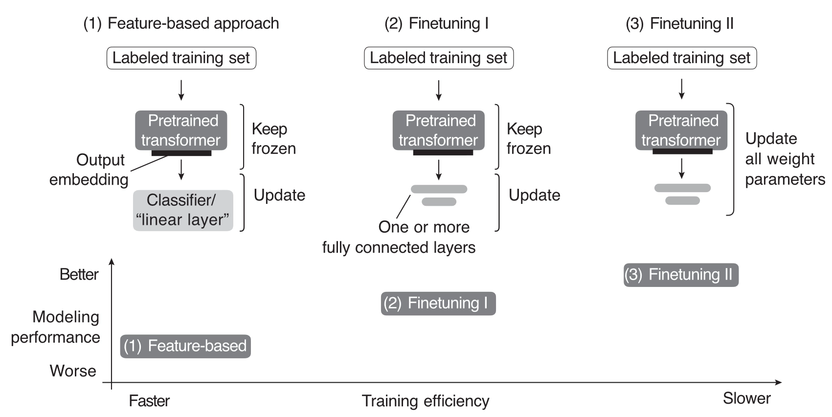
In addition to the conceptual summary of the three finetuning methods described in this section, Figure 2 also provides a rule-of-thumb guideline for these methods regarding training efficiency. Since finetuning II involves updating more layers and parameters than finetuning I, backpropagation is costlier for finetuning II. For similar reasons, finetuning II is costlier than a simpler feature-based approach.

Interested readers can find code examples illustrating the feature-based approach, finetuning one or more layers, and finetuning the complete transformer for classification here.

In-Context Learning, Indexing, and Prompt Tuning

LLMs like GPT-2 and GPT-3 popularized the concept of in-context learning, often called zero-shot or few-shot learning in this context, which is illustrated in Figure 3.

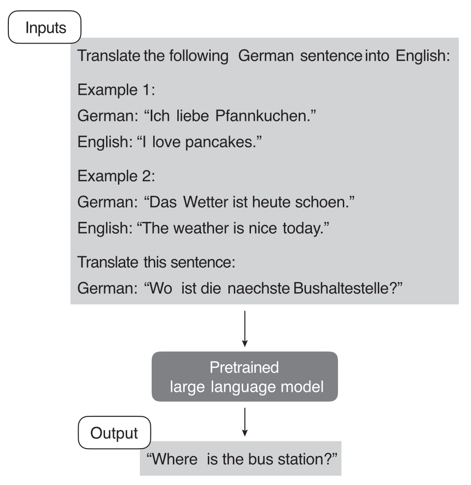
As Figure 3 shows, in-context learning aims to provide context or examples of the task within the input or prompt, allowing the model to infer the desired behavior and generate appropriate responses. This approach takes advantage of the model’s ability to learn from vast amounts of data during pretraining, which includes diverse tasks and contexts.

Note: The definition of few-shot learning, considered synonymous with in-context learning-based methods, differs from the conventional approach to few-shot learning discussed in Chapter 3.

For example, suppose we want to use in-context learning for few-shot German–English translation using a large-scale pretrained language model like GPT-3. To do so, we provide a few examples of German–English translations to help the model understand the desired task, as follows:

Translate the following German sentences into English:
Example 1:
German: "Ich liebe Pfannkuchen."
English: "I love pancakes."

Example 2:
German: "Das Wetter ist heute schoen."
English: "The weather is nice today."

Translate this sentence:
German: "Wo ist die naechste Bushaltestelle?"

Generally, in-context learning does not perform as well as finetuning for certain tasks or specific datasets since it relies on the pretrained model’s ability to generalize from its training data without further adapting its parameters for the particular task at hand.

However, in-context learning has its advantages. It can be particularly useful when labeled data for finetuning is limited or unavailable. It also enables rapid experimentation with different tasks without finetuning the model parameters in cases where we don’t have direct access to the model or where we interact only with the model through a UI or API (for example, ChatGPT).

Related to in-context learning is the concept of hard prompt tuning, where hard refers to the non-differentiable nature of the input tokens. Where the previously described finetuning methods update the model parameters to better perform the task at hand, hard prompt tuning aims to optimize the prompt itself to achieve better performance. Prompt tuning does not modify the model parameters, but it may involve using a smaller labeled dataset to identify the best prompt formulation for the specific task. For example, to improve the prompts for the previous German–English translation task, we might try the following three prompting variations:

• "Translate the German sentence '{german_sentence}' into English: {english_translation}"

• "German: '{german_sentence}' | English: {english_translation}"

• "From German to English: '{german_sentence}' -> {english_translation}"

Prompt tuning is a resource-efficient alternative to parameter finetuning. However, its performance is usually not as good as full model finetuning, as it does not update the model’s parameters for a specific task, potentially limiting its ability to adapt to task-specific nuances. Furthermore, prompt tuning can be labor intensive since it requires either human involvement comparing the quality of the different prompts or another similar method to do so. This is often known as hard prompting since, again, the input tokens are not differentiable. In addition, other methods exist that propose to use another LLM for automatic prompt generation and evaluation.

You can find code examples demonstrating prompting and in-context learning here.

Yet another way to leverage a purely in-context learning-based approach is LLM indexing, illustrated in Figure 4.

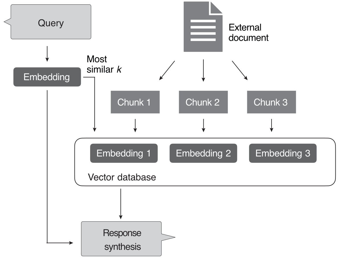
In the context of LLMs, we can think of indexing as a workaround based on in-context learning that allows us to turn LLMs into information retrieval systems to extract information from external resources and websites. In Figure 4, an indexing module parses a document or website into smaller chunks. These chunks are embedded into vectors that can be stored in a vector database. When a user submits a query, the indexing module computes the vector similarity between the embedded query and each vector stored in the database. Finally, the indexing module retrieves the top k most similar embeddings to synthesize the response.

LLM indexing is often used as an umbrella term that describes a framework or process of connecting an LLM to an existing data source. A specific example of this is retrieval augmented generation (RAG). RAG involves combining an LLM with a retrieval system to enhance the model’s ability to generate responses.

Interested readers can find code examples illustrating LLM Indexing and retrieval augmented generation here.

Parameter-Efficient Finetuning

In recent years, many methods have been developed to adapt pretrained transformers more efficiently for new target tasks. These methods are commonly referred to as parameter-efficient finetuning, with the most popular methods at the time of writing summarized in Figure 5.

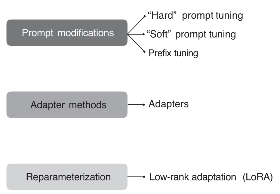
In contrast to the hard prompting approach discussed in the previous section, soft prompting strategies optimize embedded versions of the prompts. While in hard prompt tuning we modify the discrete input tokens, in soft prompt tuning we utilize trainable parameter tensors instead.

Soft Prompt Tuning

The idea behind soft prompt tuning is to prepend a trainable parameter tensor (the “soft prompt”) to the embedded query tokens. The prepended tensor is then tuned to improve the modeling performance on a target dataset using gradient descent. In Python-like pseudocode, soft prompt tuning can be described as

x = EmbeddingLayer(input_ids)
x = concatenate([soft_prompt_tensor, x],
                 dim=seq_len)
output = model(x)

where the soft_prompt_tensor has the same feature dimension as the embedded inputs produced by the embedding layer. Consequently, the modified input matrix has additional rows (as if it extended the original input sequence with additional tokens, making it longer).

Prefix Tuning

Another popular prompt tuning method is prefix tuning. Prefix tuning is similar to soft prompt tuning, except that in prefix tuning, we prepend trainable tensors (soft prompts) to each transformer block instead of only the embedded inputs, which can stabilize the training. The implementation of prefix tuning is illustrated in the following pseudocode:

def transformer_block_with_prefix(x):
    ➊ soft_prompt = FullyConnectedLayers( # Prefix
        soft_prompt)                      # Prefix
    # 2:
    ➋ x = concatenate([soft_prompt, x],   # Prefix
                       dim=seq_len)       # Prefix
    ➌ x = SelfAttention(x)
    x = LayerNorm(x + residual)
    residual = x
    x = FullyConnectedLayers(x) 
    x = LayerNorm(x + residual)
    return x      

Let’s break Listing 1 into three main parts: implementing the soft prompt, concatenating the soft prompt (prefix) with the input, and implementing the rest of the transformer block. First, the soft_prompt, a tensor, is processed through a set of fully connected layers ➊. Second, the transformed soft prompt is concatenated with the main input, x ➋. The dimension along which they are concatenated is denoted by seq_len, referring to the sequence length dimension. Third, the subsequent lines of code ➌ describe the standard operations in a transformer block, including self-attention, layer normalization, and feed-forward neural network layers, wrapped around residual connections.

As shown in Listing 1, prefix tuning modifies a transformer block by adding a trainable soft prompt. Figure 6 further illustrates the difference between a regular transformer block and a prefix tuning transformer block.

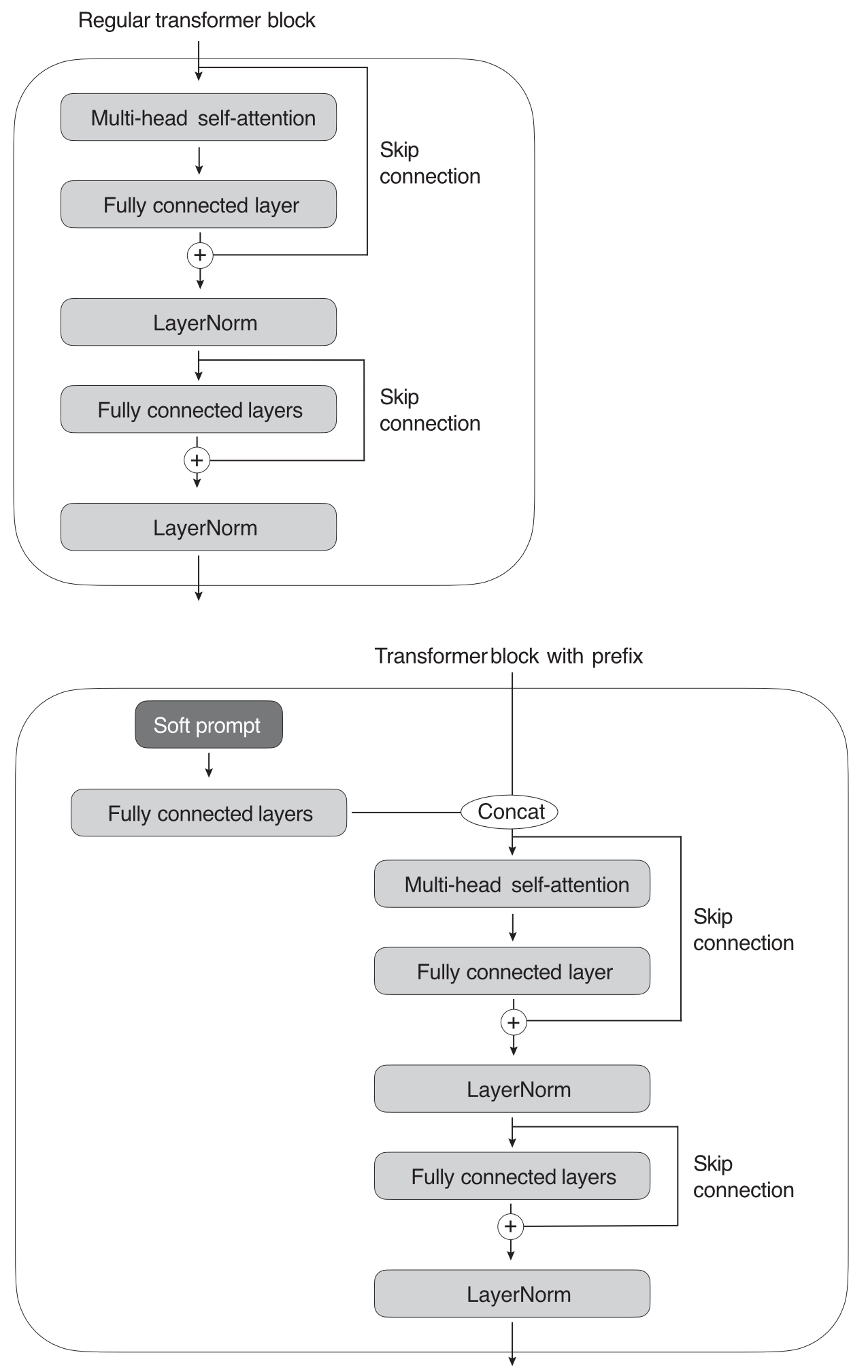
Both soft prompt tuning and prefix tuning are considered parameter efficient since they require training only the prepended parameter tensors and not the LLM parameters themselves.

Adapter Methods

Adapter methods are related to prefix tuning in that they add additional parameters to the transformer layers. In the original adapter method, additional fully connected layers were added after the multi-head self-attention and existing fully connected layers in each transformer block, as illustrated in Figure 7.

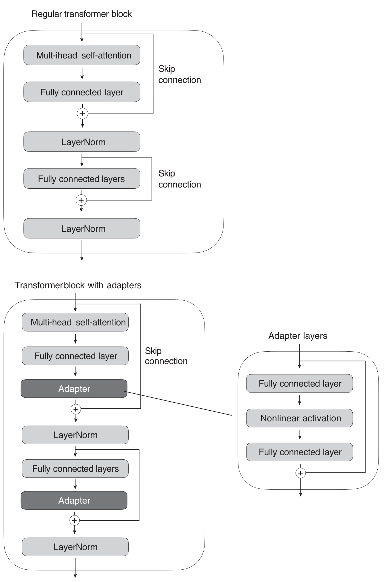
Only the new adapter layers are updated when training the LLM using the original adapter method, while the remaining transformer layers remain frozen. Since the adapter layers are usually small—the first fully connected layer in an adapter block projects its input into a low-dimensional representation, while the second layer projects it back into the original input dimension—this adapter method is usually considered parameter efficient.

In pseudocode, the original adapter method can be written as follows:

def transformer_block_with_adapter(x):
    residual = x
    x = SelfAttention(x)
    x = FullyConnectedLayers(x)  # Adapter
    x = LayerNorm(x + residual)
    residual = x
    x = FullyConnectedLayers(x)
    x = FullyConnectedLayers(x)  # Adapter
    x = LayerNorm(x + residual)
    return x

Low-rank adaptation

Low-rank adaptation (LoRA), another popular parameter-efficient finetuning method worth considering, refers to reparameterizing pretrained LLM weights using low-rank transformations. LoRA is related to the concept of low-rank transformation, a technique to approximate a high-dimensional matrix or dataset using a lower-dimensional representation. The lower-dimensional representation (or low-rank approximation) is achieved by finding a combination of fewer dimensions that can effectively capture most of the information in the original data. Popular low-rank transformation techniques include principal component analysis and singular vector decomposition.

For example, suppose \(\Delta W\) represents the parameter update for a weight matrix of the LLM with dimension \(\mathbb{R}^{A \times B}\). We can decompose the weight update matrix into two smaller matrices: \(\Delta W = W_A W_B\), where \(W_A \in \mathbb{R}^{A \times h}\) and \(W_A \in \mathbb{R}^{h \times B}\). Here, we keep the original weight frozen and train only the new matrices \(W_A\) and \(W_B\)

How is this method parameter efficient if we introduce new weight matrices? These new matrices can be very small. For example, if \(A = 25\) and \(B=50\), then the size of \(\Delta W\) is \(25 \times 50=1,250\). If \(h=5\), then \(W_A\) has 125 parameters, \(W_B\) has 250 parameters, and the two matrices combined have only \(125 + 250 = 375\) parameters in total.

After learning the weight update matrix, we can then write the matrix multiplication of a fully connected layer, as shown in this pseudocode:

def lora_forward_matmul(x):
    h = x . W  # Regular matrix multiplication
    h += x . (W_A . W_B) * scalar
    return h

In Listing 2, scalar is a scaling factor that adjusts the magnitude of the combined result (original model output plus low-rank adaptation). This balances the pretrained model’s knowledge and the new task-specific adaptation. According to the original paper introducing the LoRA method, models using LoRA perform slightly better than models using the adapter method across several task-specific benchmarks. Often, LoRA performs even better than models finetuned using the finetuning II method described earlier.

Reinforcement Learning with Human Feedback

The previous section focused on ways to make finetuning more efficient. Switching gears, how can we improve the modeling performance of LLMs via finetuning?

The conventional way to adapt or finetune an LLM for a new target domain or task is to use a supervised approach with labeled target data. For instance, the finetuning II approach allows us to adapt a pretrained LLM and finetune it on a target task such as sentiment classification, using a dataset that contains texts with sentiment labels like positive, neutral, and negative.

Supervised finetuning is a foundational step in training an LLM. An additional, more advanced step is reinforcement learning with human feedback (RLHF), which can be used to further improve the model’s alignment with human preferences. For example, ChatGPT and its predecessor, InstructGPT, are two popular examples of pretrained LLMs (GPT-3) finetuned using RLHF.

In RLHF, a pretrained model is finetuned using a combination of supervised learning and reinforcement learning. This approach was popularized by the original ChatGPT model, which was in turn based on InstructGPT. Human feedback is collected by having humans rank or rate different model outputs, providing a reward signal. The collected reward labels can be used to train a reward model that is then used to guide the LLMs’ adaptation to human preferences. The reward model is learned via supervised learning, typically using a pretrained LLM as the base model, and is then used to adapt the pretrained LLM to human preferences via additional finetuning. The training in this additional finetuning stage uses a flavor of reinforcement learning called proximal policy optimization.

RLHF uses a reward model instead of training the pretrained model on the human feedback directly because involving humans in the learning process would create a bottleneck since we cannot obtain feedback in real time.

Adapting Pretrained Language Models

While finetuning all layers of a pretrained LLM remains the gold standard for adaption to new target tasks, several efficient alternatives exist for leveraging pretrained transformers. For instance, we can effectively apply LLMs to new tasks while minimizing computational costs and resources by utilizing feature-based methods, in-context learning, or parameter-efficient finetuning techniques.

The three conventional methods—feature-based approach, finetuning I, and finetuning II—provide different computational efficiency and performance trade-offs. Parameter-efficient finetuning methods like soft prompt tuning, prefix tuning, and adapter methods further optimize the adaptation process, reducing the number of parameters to be updated. Meanwhile, RLHF presents an alternative approach to supervised finetuning, potentially improving modeling performance.

In sum, the versatility and efficiency of pretrained LLMs continue to advance, offering new opportunities and strategies for effectively adapting these models to a wide array of tasks and domains. As research in this area progresses, we can expect further improvements and innovations in using pretrained language models.

References and Further Reading

1. The paper introducing the GPT-2 model: Alec Radford et al., “Language Models Are Unsupervised Multitask Learners” (2019), https://www.semanticscholar.org/paper/Language-Models-are-Unsupervised-Multitask-Learners-Radford-Wu/9405cc0d6169988371b2755e573cc28650d14dfe.
2. The paper introducing the GPT-3 model: Tom B. Brown et al., “Language Models Are Few-Shot Learners” (2020), https://arxiv.org/abs/2005.14165.
3. The automatic prompt engineering method, which proposes using another LLM for automatic prompt generation and evaluation: Yongchao Zhou et al., “Large Language Models Are Human-Level Prompt Engineers” (2023), https://arxiv.org/abs/2211.01910.
4. LlamaIndex is an example of an indexing approach that leverages in-context learning: https://github.com/jerryjliu/llama_index.
5. DSPy is another popular open source library for LLM applications, such as retrieval augmentation and indexing: https://github.com/stanfordnlp/dspy.
6. A first instance of soft prompting: Brian Lester, Rami Al-Rfou, and Noah Constant, “The Power of Scale for Parameter-Efficient Prompt Tuning” (2021), https://arxiv.org/abs/2104.08691.
7. The paper that first described prefix tuning: Xiang Lisa Li and Percy Liang, “Prefix-Tuning: Optimizing Continuous Prompts for Generation” (2021), https://arxiv.org/abs/2101.00190.
8. The paper introducing the original adapter method: Neil Houlsby et al., “Parameter-Efficient Transfer Learning for NLP” (2019), https://arxiv.org/abs/1902.00751.
9. The paper introducing the LoRA method: Edward J. Hu et al., “LoRA: Low-Rank Adaptation of Large Language Models” (2021), https://arxiv.org/abs/2106.09685.
10. A survey of more than 40 research papers covering parameterefficient finetuning methods: Vladislav Lialin, Vijeta Deshpande, and Anna Rumshisky, “Scaling Down to Scale Up: A Guide to Parameter-Efficient Fine-Tuning” (2023), https://arxiv.org/abs/2303.15647.
11. The InstructGPT paper: Long Ouyang et al., “Training Language Models to Follow Instructions with Human Feedback” (2022), https://arxiv.org/abs/2203.02155.
12. Proximal policy optimization, which is used for reinforcement learning with human feedback: John Schulman et al., “Proximal Policy Optimization Algorithms” (2017), https://arxiv.org/abs/1707.06347.
13. An article by the author describing reinforcement learning with human feedback (RLHF) and its alternatives, https://magazine.sebastianraschka.com/p/llm-training-rlhf-and-its-alternatives

Code Examples

• Feature-extractor vs. finetuning different output vs finetuning all layers
• In-context learning and prompt tuning
• Indexing and retrieval augmented generation (RAG)
• Adapter finetuning
• Low-rank adaptation (LoRA) finetuning

Exercises

1. When does it make more sense to use in-context learning rather than finetuning, and vice versa?

2. In prefix tuning, adapters, and LoRA, how can we ensure that the model preserves (and does not forget) the original knowledge?

Machine Learning Q and AI

I hope you liked this excerpt! If you are interested in 29 other topics related to machine learning and AI, you can find the book on the publisher’s website, Amazon, and many other book stores.

Ahead of AI is a personal passion project that does not offer direct compensation, and I’d appreciate it if you’d consider purchasing a copy of my book to support these endeavors.