Improving LoRA: Implementing Weight-Decomposed Low-Rank Adaptation (DoRA) from Scratch

Low-rank adaptation (LoRA) is a machine learning technique that modifies a pretrained model (for example, an LLM or vision transformer) to better suit a specific, often smaller, dataset by adjusting only a small, low-rank subset of the model’s parameters.

This approach is important because it allows for efficient finetuning of large models on task-specific data, significantly reducing the computational cost and time required for finetuning.

Last week, researchers proposed DoRA: Weight-Decomposed Low-Rank Adaptation, a new alternative to LoRA, which may outperform LoRA by a large margin.

To understand how these methods work, we will implement both LoRA and DoRA in PyTorch from scratch in this article!

LoRA Recap

Before we dive into DoRA, here’s a brief recap of how LoRA works.

Since LLMs are large, updating all model weights during training can be expensive due to GPU memory limitations. Suppose we have a large weight matrix \(W\) for a given layer. During backpropagation, we learn a \(ΔW\) matrix, which contains information on how much we want to update the original weights to minimize the loss function during training.

In regular training and finetuning, the weight update is defined as follows:

The LoRA method proposed by Hu et al. offers a more efficient alternative to computing the weight updates \(ΔW\) by learning an approximation of it, \(ΔW ≈ AB\). In other words, in LoRA, we have the following, where \(A\) and \(B\) are two small weight matrices:

(The “.” in “\(A.B\)” stands for matrix multiplication.)

The figure below illustrates these formulas for full finetuning and LoRA side by side.

How does LoRA save GPU memory? If a pretrained weight matrix \(W\) is a 1,000×1,000 matrix, then the weight update matrix \(ΔW\) in regular finetuning is a 1,000×1,000 matrix as well. In this case, \(ΔW\) has 1,000,000 parameters. If we consider a LoRA rank of 2, then \(A\) is a 1000×2 matrix, and \(B\) is a 2×1000 matrix, and we only have 2×2×1,000 = 4,000 parameters that we need to update when using LoRA. In the previous example, with a rank of 2, that’s 250 times fewer parameters.

Of course, \(A\) and \(B\) can’t capture all the information that \(ΔW\) could capture, but this is by design. When using LoRA, we hypothesize that the model requires W to be a large matrix with full rank to capture all the knowledge in the pretraining dataset. However, when we finetune an LLM, we don’t need to update all the weights and capture the core information for the adaptation in a smaller number of weights than \(ΔW\) would; hence, we have the low-rank updates via \(AB\).

If you paid close attention, the full finetuning and LoRA depictions in the figure above look slightly different from the formulas I have shown earlier. That’s due to the distributive law of matrix multiplication: we don’t have to add the weights with the updated weights but can keep them separate. For instance, if \(x\) is the input data, then we can write the following for regular finetuning:

Similarly, we can write the following for LoRA:

The fact that we can keep the LoRA weight matrices separate makes LoRA especially attractive. In practice, this means that we don’t have to modify the weights of the pretrained model at all, as we can apply the LoRA matrices on the fly. This is especially useful if you are considering hosting a model for multiple customers. Instead of having to save the large updated models for each customer, you only have to save a small set of LoRA weights alongside the original pretrained model.

To make this less abstract and to provide additional intuition, we will implement LoRA in code from scratch in the next section.

A LoRA Layer Code Implementation

We begin by initializing a LoRALayer that creates the matrices A and B, along with the alpha scaling hyperparameter and the rank hyperparameters. This layer can accept an input and compute the corresponding output, as illustrated in the figure below.

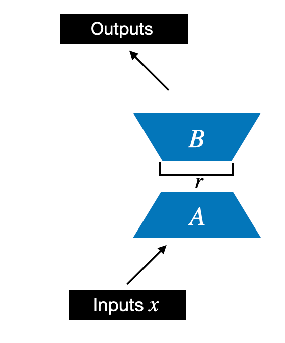
In code, this LoRA layer depicted in the figure above looks like as follows:

import torch.nn as nn

class LoRALayer(nn.Module):
    def __init__(self, in_dim, out_dim, rank, alpha):
        super().__init__()
        std_dev = 1 / torch.sqrt(torch.tensor(rank).float())
        self.A = nn.Parameter(torch.randn(in_dim, rank) * std_dev)
        self.B = nn.Parameter(torch.zeros(rank, out_dim))
        self.alpha = alpha

    def forward(self, x):
        x = self.alpha * (x @ self.A @ self.B)
        return x

In the code above, rank is a hyperparameter that controls the inner dimension of the matrices A and B. In other words, this parameter controls the number of additional parameters introduced by LoRA and is a key factor in determining the balance between model adaptability and parameter efficiency.

The second hyperparameter, alpha, is a scaling hyperparameter applied to the output of the low-rank adaptation. It essentially controls the extent to which the adapted layer’s output is allowed to influence the original output of the layer being adapted. This can be seen as a way to regulate the impact of the low-rank adaptation on the layer’s output.

So far, the LoRALayer class we implemented above allows us to transform the layer inputs x. However, in LoRA, we are usually interested in replacing existing Linear layers so that the weight update is applied to the existing pretrained weights, as shown in the figure below:

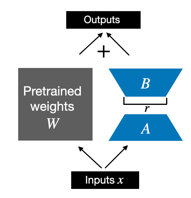
To incorporate the original Linear layer weights as shown in the figure above, we will implement a LinearWithLoRA layer that uses the previously implemented LoRALayer and can be used to replace existing Linear layers in a neural network, for example, the self-attention module or feed forward modules in an LLM:

class LinearWithLoRA(nn.Module):

    def __init__(self, linear, rank, alpha):
        super().__init__()
        self.linear = linear
        self.lora = LoRALayer(
            linear.in_features, linear.out_features, rank, alpha
        )

    def forward(self, x):
        return self.linear(x) + self.lora(x)

Note that since we initialize the weight matrix B (self.B in LoraLayer) with zero values in the LoRA layer, the matrix multiplication between A and B results in a matrix consisting of 0’s and doesn’t affect the original weights (since adding 0 to the original weights does not modify them).

Let’s try out LoRA on a small neural network layer represented by a single Linearlayer:

In:

torch.manual_seed(123)
layer = nn.Linear(10, 2)
x = torch.randn((1, 10))

print("Original output:", layer(x))

Out:

Original output: tensor([[0.6639, 0.4487]], grad_fn=<AddmmBackward0>)

Now, applying LoRA to the Linear layer, we see that the results are the same since we haven’t trained the LoRA weights yet. In other words, everything works as expected:

In:

layer_lora_1 = LinearWithLoRA(layer, rank=2, alpha=4)
print("LoRA output:", layer_lora_1(x))

Out:

LoRA output: tensor([[0.6639, 0.4487]], grad_fn=<AddmmBackward0>)

Earlier, I mentioned the distributive law of matrix multiplication:

\(x.(W+A.B) = x.W + x.A.B\).

Here, this means that we can also combine or merge the LoRA matrices and original weights, which should result in an equivalent implementation. In code, this alternative implementation to the LinearWithLoRA layer looks as follows:

class LinearWithLoRAMerged(nn.Module):
    def __init__(self, linear, rank, alpha):
        super().__init__()
        self.linear = linear
        self.lora = LoRALayer(
            linear.in_features, linear.out_features, rank, alpha
        )

    def forward(self, x):
        lora = self.lora.A @ self.lora.B # Combine LoRA matrices
        # Then combine LoRA with orig. weights
        combined_weight = self.linear.weight + self.lora.alpha*lora.T
        return F.linear(x, combined_weight, self.linear.bias)

In short, LinearWithLoRAMerged computes the left side of the equation \(x.(W+A.B) = x.W + x.A.B\) whereas LinearWithLoRA computes the right side – both are equivalent.

We can verify that this results in the same outputs as before via the following code:

In:

layer_lora_2 = LinearWithLoRAMerged(layer, rank=2, alpha=4)
print("LoRA output:", layer_lora_2(x))

Out:

LoRA output: tensor([[0.6639, 0.4487]], grad_fn=<AddmmBackward0>)

Now that we have a working LoRA implementation let’s see how we can apply it to a neural network in the next section.

Applying LoRA Layers

Why did we implement LoRA in the manner described above using PyTorch modules? This approach enables us to easily replace a Linear layer in an existing neural network (for example, the feed forward or attention modules of a Large Language Model) with our new LinearWithLoRA (or LinearWithLoRAMerged) layers.

For simplicity, let’s focus on a small 3-layer multilayer perceptron instead of an LLM for now, which is illustrated in the figure below:

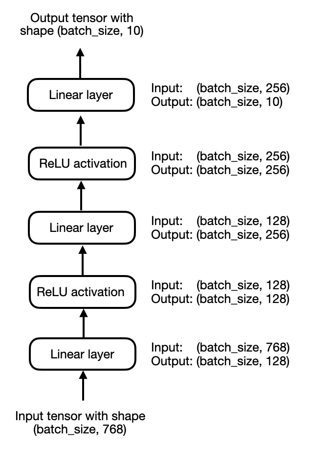
In code, we can implement the multilayer perceptron, shown above, as follows:

In:

class MultilayerPerceptron(nn.Module):
    def __init__(self, num_features,
        num_hidden_1, num_hidden_2, num_classes):
        super().__init__()
        self.layers = nn.Sequential(
            nn.Linear(num_features, num_hidden_1),
            nn.ReLU(),
            nn.Linear(num_hidden_1, num_hidden_2),
            nn.ReLU(),

            nn.Linear(num_hidden_2, num_classes)
        )

    def forward(self, x):
        x = self.layers(x)
        return x


model = MultilayerPerceptron(
    num_features=num_features,
    num_hidden_1=num_hidden_1,
    num_hidden_2=num_hidden_2,
    num_classes=num_classes
)

print(model)

Out:

MultilayerPerceptron(
  (layers): Sequential(
    (0): Linear(in_features=784, out_features=128, bias=True)
    (1): ReLU()
    (2): Linear(in_features=128, out_features=256, bias=True)
    (3): ReLU()
    (4): Linear(in_features=256, out_features=10, bias=True)
  )
)

Using LinearWithLora, we can then add the LoRA layers by replacing the original Linear layers in the multilayer perceptron model:

In:

model.layers[0] = LinearWithLoRA(model.layers[0], rank=4, alpha=8)
model.layers[2] = LinearWithLoRA(model.layers[2], rank=4, alpha=8)
model.layers[4] = LinearWithLoRA(model.layers[4], rank=4, alpha=8)

print(model)

Out:

MultilayerPerceptron(
  (layers): Sequential(
    (0): LinearWithLoRA(
      (linear): Linear(in_features=784, out_features=128, bias=True)
      (lora): LoRALayer()
    )
    (1): ReLU()
    (2): LinearWithLoRA(
      (linear): Linear(in_features=128, out_features=256, bias=True)
      (lora): LoRALayer()
    )
    (3): ReLU()
    (4): LinearWithLoRA(
      (linear): Linear(in_features=256, out_features=10, bias=True)
      (lora): LoRALayer()
    )
  )
)

Then, we can freeze the original Linear layers and only make the LoRALayer layers trainable, as follows:

In:

def freeze_linear_layers(model):
    for child in model.children():
        if isinstance(child, nn.Linear):
            for param in child.parameters():
                param.requires_grad = False
        else:
            # Recursively freeze linear layers in children modules
            freeze_linear_layers(child)

freeze_linear_layers(model)
for name, param in model.named_parameters():
    print(f"{name}: {param.requires_grad}")

Out:

layers.0.linear.weight: False
layers.0.linear.bias: False
layers.0.lora.A: True
layers.0.lora.B: True
layers.2.linear.weight: False
layers.2.linear.bias: False
layers.2.lora.A: True
layers.2.lora.B: True
layers.4.linear.weight: False
layers.4.linear.bias: False
layers.4.lora.A: True
layers.4.lora.B: True

Based on the True and False values above, we can visually confirm that only the LoRA layers are trainable now (True means trainable, False means frozen). In practice, we would then train the network with this LoRA configuration on a new dataset or task.

To avoid making this a very long article, I am skipping over the boilerplate code to train this model. But if you are interested in the full code, you can find a standalone code notebook here: https://github.com/rasbt/dora-from-scratch.

Furthermore, if you are interested in a LoRA from scratch explanation and application to an LLM, also check out my Lightning Studio LoRA From Scratch – Implement Low-Rank Adaptation for LLMs in PyTorch.

Understanding Weight-Decomposed Low-Rank Adaptation (DoRA)

You may have noticed that we spent a lot of time implementing and talking about LoRA. That’s because DoRA (Weight-Decomposed Low-Rank Adaptation) can be seen as an improvement or extension of LoRA that is built on top of it, and we can now easily adapt some of our previous code to implement DoRA.

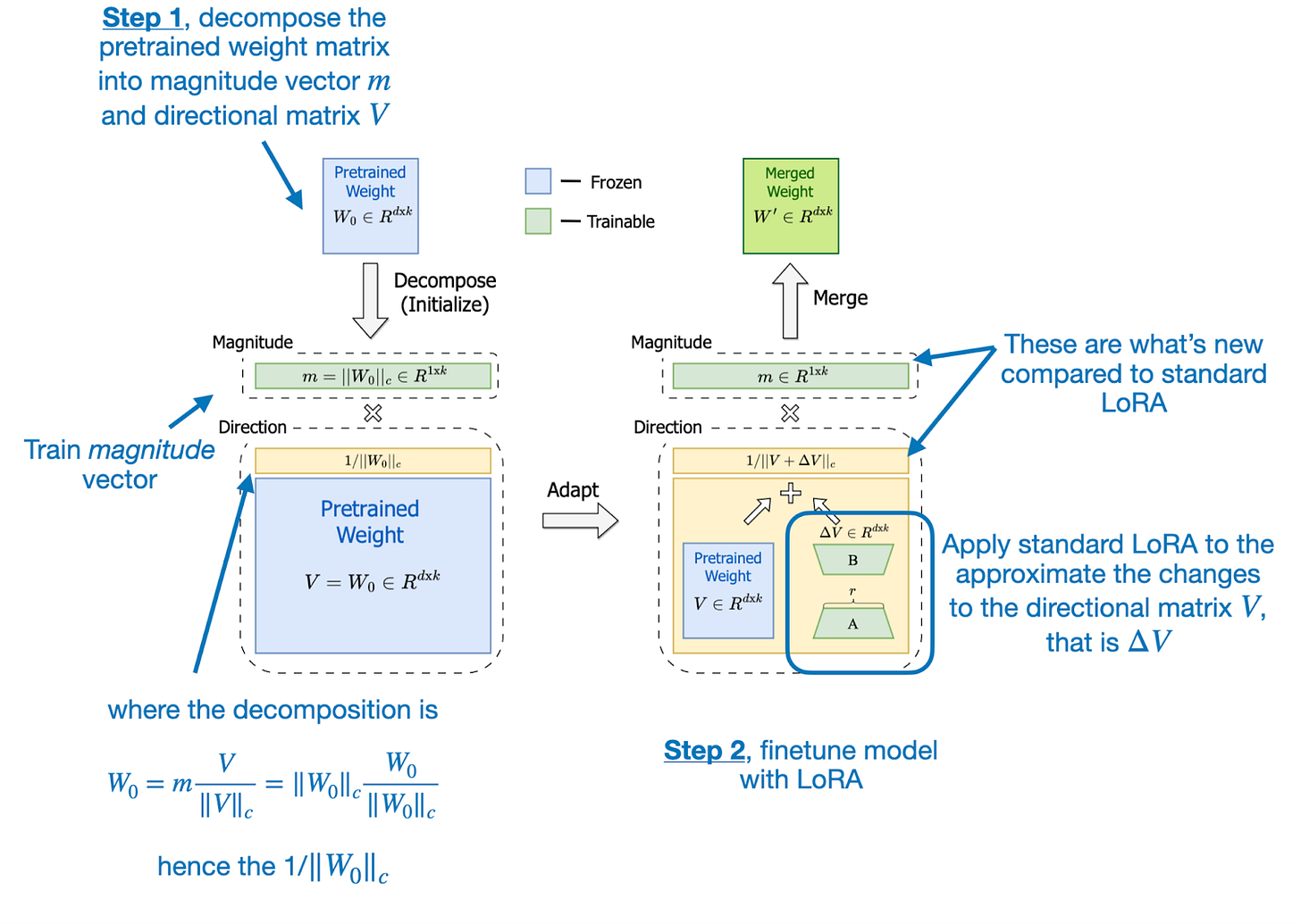
DoRA can be described in two steps, where the first step is to decompose a pretrained weight matrix into a magnitude vector (\(m\)) and a directional matrix (\(V\)). The second step is applying LoRA to the directional matrix \(V\) and training the magnitude vector \(m\) separately.

The decomposition into magnitude and directional components is inspired by the mathematical principle that any vector can be represented as the product of its magnitude (a scalar value indicating its length) and its direction (a unit vector indicating its orientation in space).

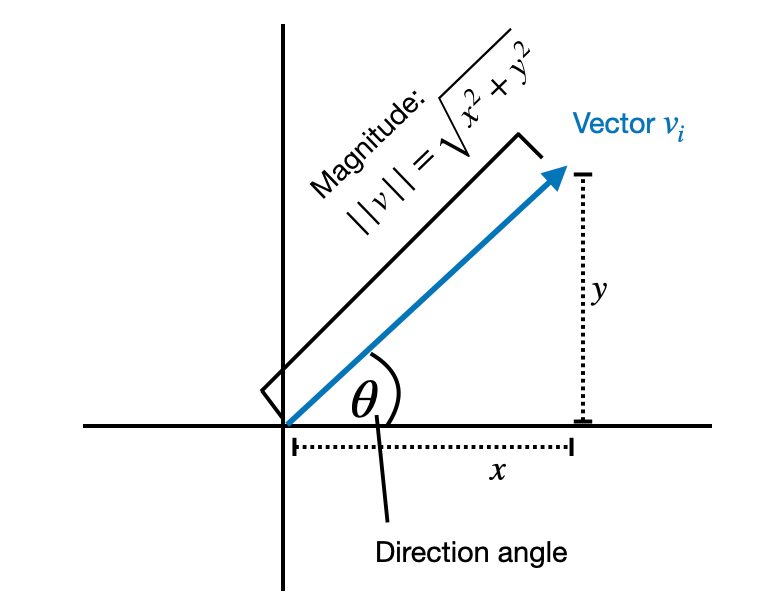
For example, if have a 2D vector [1, 2], we can decompose it into a magnitude 2.24 and a directional vector \([0.447, 0.894]\). Then \(2.24 \times [0.447, 0.894] = [1, 2]\).

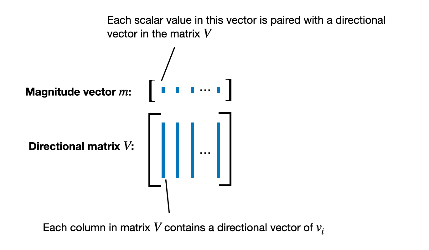
In DoRA, we apply the decomposition into magnitude and directional components to a whole pretrained weight matrix \(W\) instead of a vector, where each column (vector) of the weight matrix corresponds to the weights connecting all inputs to a particular output neuron.

So, the result of decomposing \(W\) is a magnitude vector \(m\) that represents the scale or length of each column vector in the weight matrix, as illustrated in the figure below.

Then, DoRA takes the directional matrix \(V\) and applies standard LoRA, for instance:

The normalization, which I abbreviated as “norm” to not further complicate things in this overview, is based on the weight normalization method proposed in Saliman’s and Kingma’s 2016 Weight Normalization: A Simple Reparameterization to Accelerate Training of Deep Neural Networks paper.

The DoRA two-step process (decomposing a pretrained weight matrix and applying LoRA to the directional matrix) is further illustrated in the figure from the DoRA paper below.

The motivation for developing DoRA is based on analyzing and comparing the LoRA and full finetuning learning patterns. The DoRA authors found that LoRA either increases or decreases magnitude and direction updates proportionally but seems to lack the capability to make only subtle directional changes as found in full finetuning. Hence, the researchers propose the decoupling of magnitude and directional components.

In other words, their DoRA method aims to apply LoRA only to the directional component, \(V\), while also allowing the magnitude component, \(m\), to be trained separately.

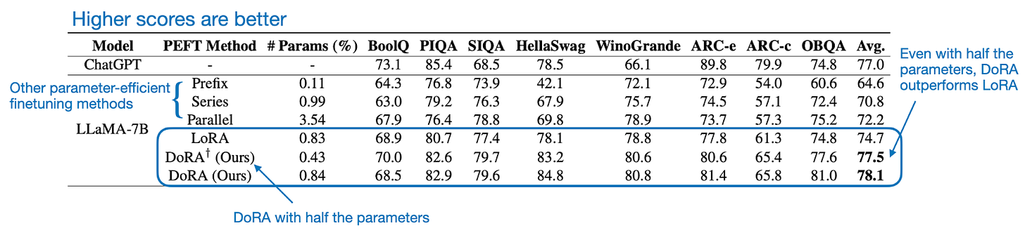
Introducing the magnitude vector m adds 0.01% more parameters if DoRA is compared to LoRA. However, across both LLM and vision transformer benchmarks, they found that DoRA even outperforms LoRA if the DoRA rank is halved, for instance, when DoRA only uses half the parameters of regular LoRA, as shown in the performance comparison below.

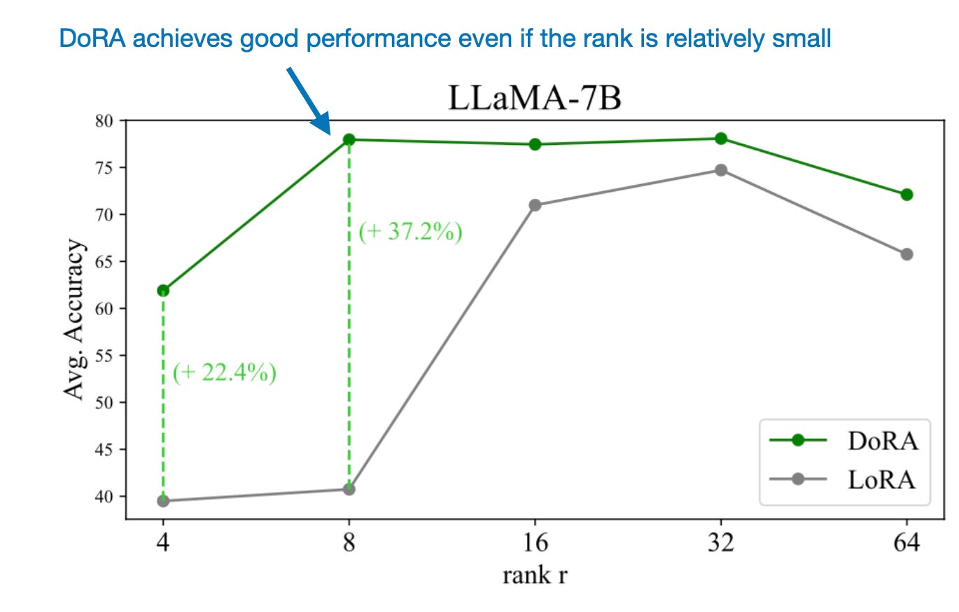
As I wrote in another article a few months ago, LoRA requires careful tuning of the rank to optimize performance: Practical Tips for Finetuning LLMs Using LoRA (Low-Rank Adaptation). However, DoRA seems to be much more robust to changes in rank, as shown in the comparison below.

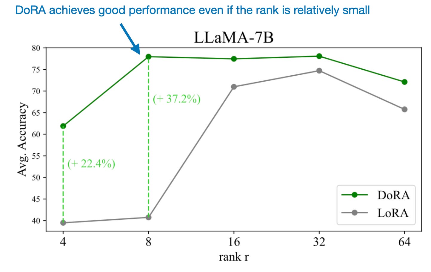
The possibility to successfully use DoRA with relatively small ranks makes this method even more parameter-efficient than LoRA.

Overall, I am quite impressed by the results, and it should not be too big of a lift to upgrade a LoRA implementation to DoRA, which we will do in the next section.

Implementing DoRA Layers in PyTorch

In this section, we will see what DoRA looks like in code. Previously, we said that we can initialize a pretrained weight \(W_0\) with magnitude \(m\) and directional component \(V\). For instance, we have the following equation:

where \(\|V\|_c\) is the vector-wise norm of \(V\). Then we can write DoRA including the LoRA weight update \(BA\) as shown below:

Now, in the DoRA paper, the authors formulate DoRA as follows, where they use the initial pretrained weights \(W_0\) as the directional component directly and learn magnitude vector \(m\) during training:

Here, \(ΔV\) is the update to the directional component, matrix \(V\).

While the original authors haven’t released the official implementation yet, you can find an independent implementation here, which loosely inspired my implementation below

Taking our previous LinearWithLoRAMerged implementation, we can upgrade it to DoRA as follows:

class LinearWithDoRAMerged(nn.Module):

    def __init__(self, linear, rank, alpha):
        super().__init__()
        self.linear = linear
        self.lora = LoRALayer(
            linear.in_features, linear.out_features, rank, alpha
        )
        self.m = nn.Parameter(
            self.linear.weight.norm(p=2, dim=0, keepdim=True))


  # Code loosely inspired by
  # https://github.com/catid/dora/blob/main/dora.py

    def forward(self, x):
        lora = self.lora.A @ self.lora.B
        numerator = self.linear.weight + self.lora.alpha*lora.T
        denominator = numerator.norm(p=2, dim=0, keepdim=True)
        directional_component = numerator / denominator
        new_weight = self.m * directional_component
        return F.linear(x, new_weight, self.linear.bias)

The LinearWithDoRAMerged class is different from our previous LinearWithLoRAMerged class in several key aspects, primarily in how it modifies and applies the weights of the Linear layer. However, both classes integrate a LoRALayer to augment the original linear layer’s weights, but DoRA adds weight normalization and adjustment.

The figure below shows a file-diff of both classes side by side:

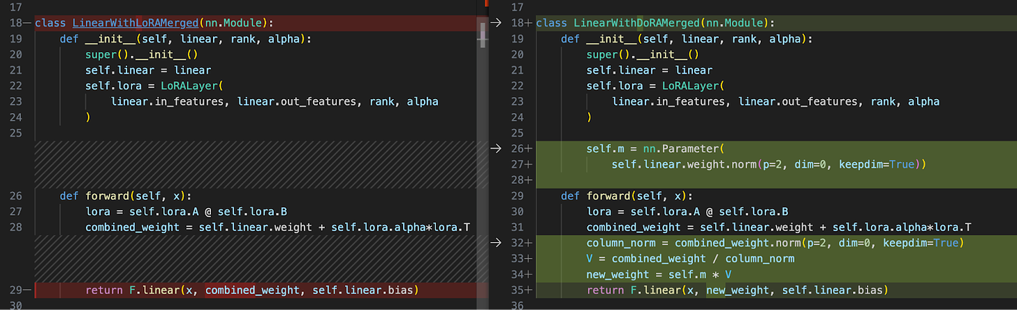
As we can see in the figure above, LinearWithDoRAMerged introduces an additional step involving dynamic normalization of the augmented weights.

After combining the original weights with the LoRA-adjusted weights (self.linear.weight + self.lora.alpha*lora.T), it calculates the norm of these combined weights across columns (column_norm). Then, it normalizes the combined weights by dividing them by their norms (V = combined_weight / column_norm). This step ensures that each column of the combined weight matrix has a unit norm, which can help stabilize the learning process by maintaining the scale of weight updates.

DoRA also introduces a learnable vector self.m, which represents the magnitude of each column of the normalized weight matrix. This parameter allows the model to dynamically adjust the scale of each weight vector in the combined weight matrix during training. This additional flexibility can help the model better capture the importance of different features.

In summary, LinearWithDoRAMerged extends the concept of LinearWithLoRAMerged by incorporating dynamic weight normalization and scaling to improve the training performance.

In practice, considering the multilayer perceptron from earlier, we can simply swap existing Linear layers with our LinearWithDoRAMerged layers as follows:

In:

model.layers[0] = LinearWithDoRAMerged(model.layers[0], rank=4, alpha=8)
model.layers[2] = LinearWithDoRAMerged(model.layers[2], rank=4, alpha=8)
model.layers[4] = LinearWithDoRAMerged(model.layers[4], rank=4, alpha=8)

print(model)

Out:

MultilayerPerceptron(
  (layers): Sequential(
    (0): LinearWithDoRAMerged(
      (linear): Linear(in_features=784, out_features=128, bias=True)
      (lora): LoRALayer()
    )
    (1): ReLU()
    (2): LinearWithDoRAMerged(
      (linear): Linear(in_features=128, out_features=256, bias=True)
      (lora): LoRALayer()
    )
    (3): ReLU()
    (4): LinearWithDoRAMerged(
      (linear): Linear(in_features=256, out_features=10, bias=True)
      (lora): LoRALayer()
    )
  )
)

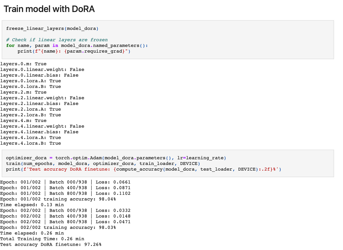
Before we finetune the model, we can reuse the freeze_linear_layers function we implemented earlier to only make the LoRA weights and magnitude vectors trainable:

In:

freeze_linear_layers(model)
for name, param in model.named_parameters():
    print(f"{name}: {param.requires_grad}")

Out:

layers.0.m: True
layers.0.linear.weight: False
layers.0.linear.bias: False
layers.0.lora.A: True
layers.0.lora.B: True
layers.2.m: True
layers.2.linear.weight: False
layers.2.linear.bias: False
layers.2.lora.A: True
layers.2.lora.B: True
layers.4.m: True
layers.4.linear.weight: False
layers.4.linear.bias: False
layers.4.lora.A: True
layers.4.lora.B: True

The full code example, including model training, is available in my GitHub repo here: https://github.com/rasbt/dora-from-scratch.

Conclusion

In my opinion, DoRA seems like a logical, effective, and promising extension of LoRA, and I am excited to try it in real-world LLM finetuning contexts.

In the meantime, I also added the DoRA implementation above to the LoRA From Scratch – Implement Low-Rank Adaptation for LLMs in PyTorch Lightning Studio to finetune a DistilBERT language model (see bonus_02_finetune-with-dora.ipynb). Even without hyperparameter tuning, I already saw a >1% prediction accuracy improvement over LoRA.