Building A GPT-Style LLM Classifier From Scratch

In this article, I want to show you how to transform pretrained large language models (LLMs) into strong text classifiers.

But why focus on classification? First, finetuning a pretrained model for classification offers a gentle yet effective introduction to model finetuning. Second, many real-world and business challenges revolve around text classification: spam detection, sentiment analysis, customer feedback categorization, topic labeling, and more.

Announcing My New Book

I’m thrilled to announce the release of my new book, Build a Large Language Model From Scratch, published by Manning. This book, which has been nearly two years in the making, is now finally available as ebook and print version on the Manning website (with preorders also available on Amazon).

• Manning link
• Amazon link (preorder)

From my experience, the best way to deeply understand a concept is to build it from scratch. And this book guides you through the entire process of building a GPT-like LLM—from implementing data inputs to finetuning with instruction data. My goal is that, after reading this book, you’ll have a deep, detailed and thorough understanding of how LLMs work.

What You’ll Learn in This Article

To celebrate the book’s release, I’m sharing an excerpt from one of the chapters that walks you through how to finetune a pretrained LLM as a spam classifier.

Important Note

The chapter on classification finetuning is 35 pages long—too long for a single article. So, in this post, I’ll focus on a ~10-page subset that introduces the context and core concepts behind classification finetuning.

Additionally, I’ll share insights from some extra experiments that aren’t included in the book and address common questions readers might have. (Please note that the excerpt below is based on my personal draft before Manning’s professional text editing and final figure design.)

The full code for this excerpt can be found here on GitHub.

In addition, I’ll also answer 7 questions you might have regarding training LLM classifiers:

1. Do we need to train all layers?
2. Why finetuning the last token, not the first token?
3. How does BERT compare to GPT performance-wise?
4. Should we disable the causal mask?
5. What impact does increasing the model size have?
6. What improvements can we expect from LoRA?
7. Padding or no padding?

Happy reading!

Different categories of finetuning

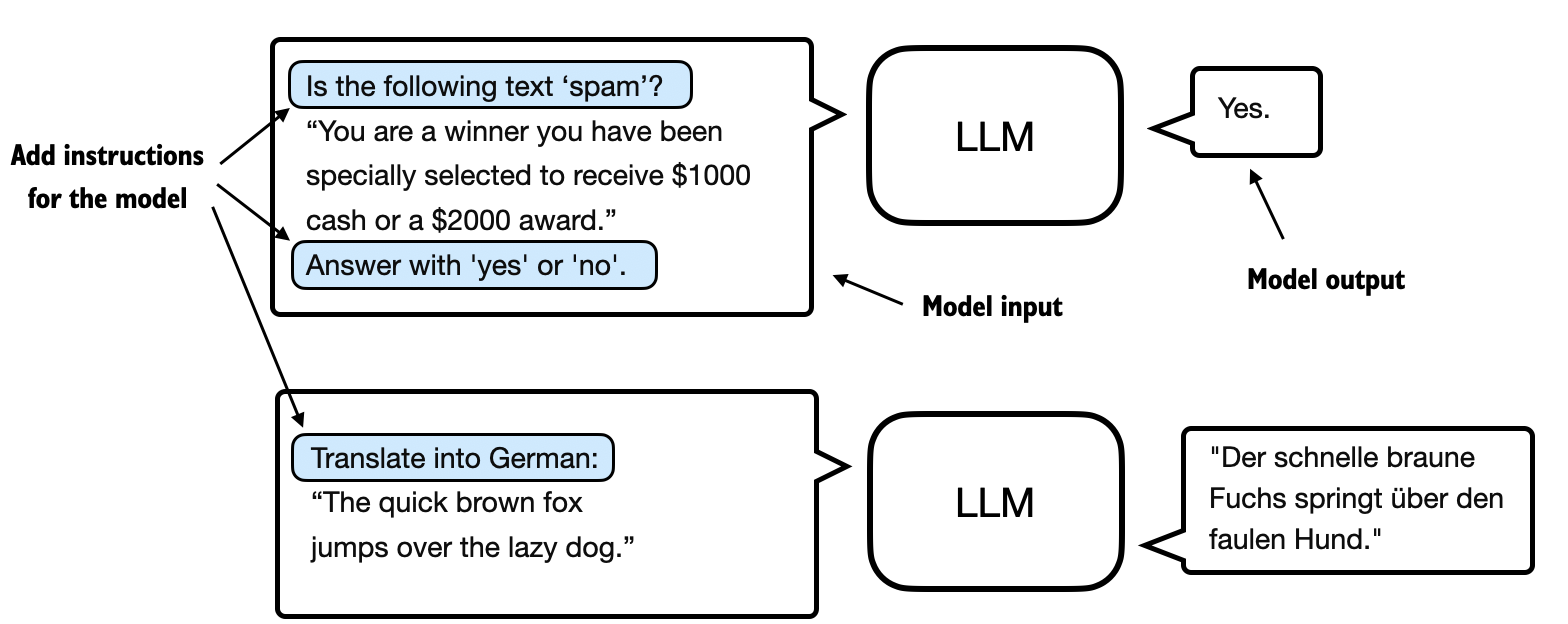
The most common ways to finetune language models are instruction finetuning and classification finetuning. Instruction finetuning involves training a language model on a set of tasks using specific instructions to improve its ability to understand and execute tasks described in natural language prompts, as illustrated in Figure 1 below.

The next chapter will discuss instruction finetuning, as illustrated in Figure 1 above. Meanwhile, this chapter is centered on classification finetuning, a concept you might already be acquainted with if you have a background in machine learning.

In classification finetuning, the model is trained to recognize a specific set of class labels, such as “spam” and “not spam.” Examples of classification tasks extend beyond large language models and email filtering; they include identifying different species of plants from images, categorizing news articles into topics like sports, politics, or technology, and distinguishing between benign and malignant tumors in medical imaging.

The key point is that a classification-finetuned model is restricted to predicting classes it has encountered during its training—for instance, it can determine whether something is “spam” or “not spam,” as illustrated in Figure 2 below, but it can’t say anything else about the input text.

In contrast to the classification-finetuned model depicted in Figure 2, an instruction-finetuned model typically has the capability to undertake a broader range of tasks. We can view a classification-finetuned model as highly specialized, and generally, it is easier to develop a specialized model than a generalist model that works well across various tasks.

Choosing the right approach

Instruction finetuning improves a model’s ability to understand and generate responses based on specific user instructions. Instruction finetuning is best suited for models that need to handle a variety of tasks based on complex user instructions, improving flexibility and interaction quality. Classification finetuning, on the other hand, is ideal for projects requiring precise categorization of data into predefined classes, such as sentiment analysis or spam detection.

While instruction finetuning is more versatile, it demands larger datasets and greater computational resources to develop models proficient in various tasks. In contrast, classification finetuning requires less data and compute power, but its use is confined to the specific classes on which the model has been trained.

Initializing a model with pretrained weights

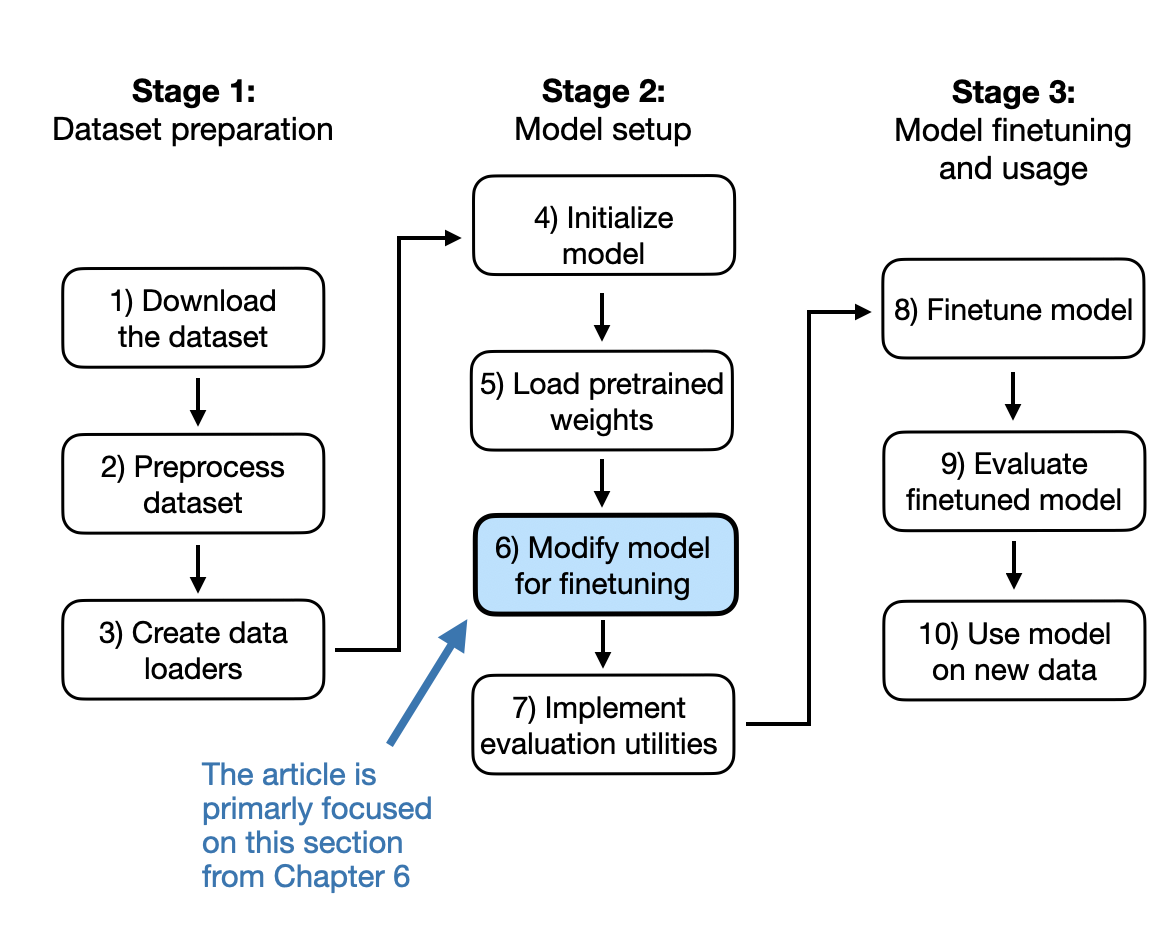
Since this is an excerpt, we’ll skip over the data preparation parts and the model’s initialization, which were implemented and pretrained in previous chapters. From my experience, maintaining focus while reading lengthy digital articles can be challenging compared to physical books. So, I’ll try to keep this excerpt/article tightly focused on one of the key takeaways from this chapter.

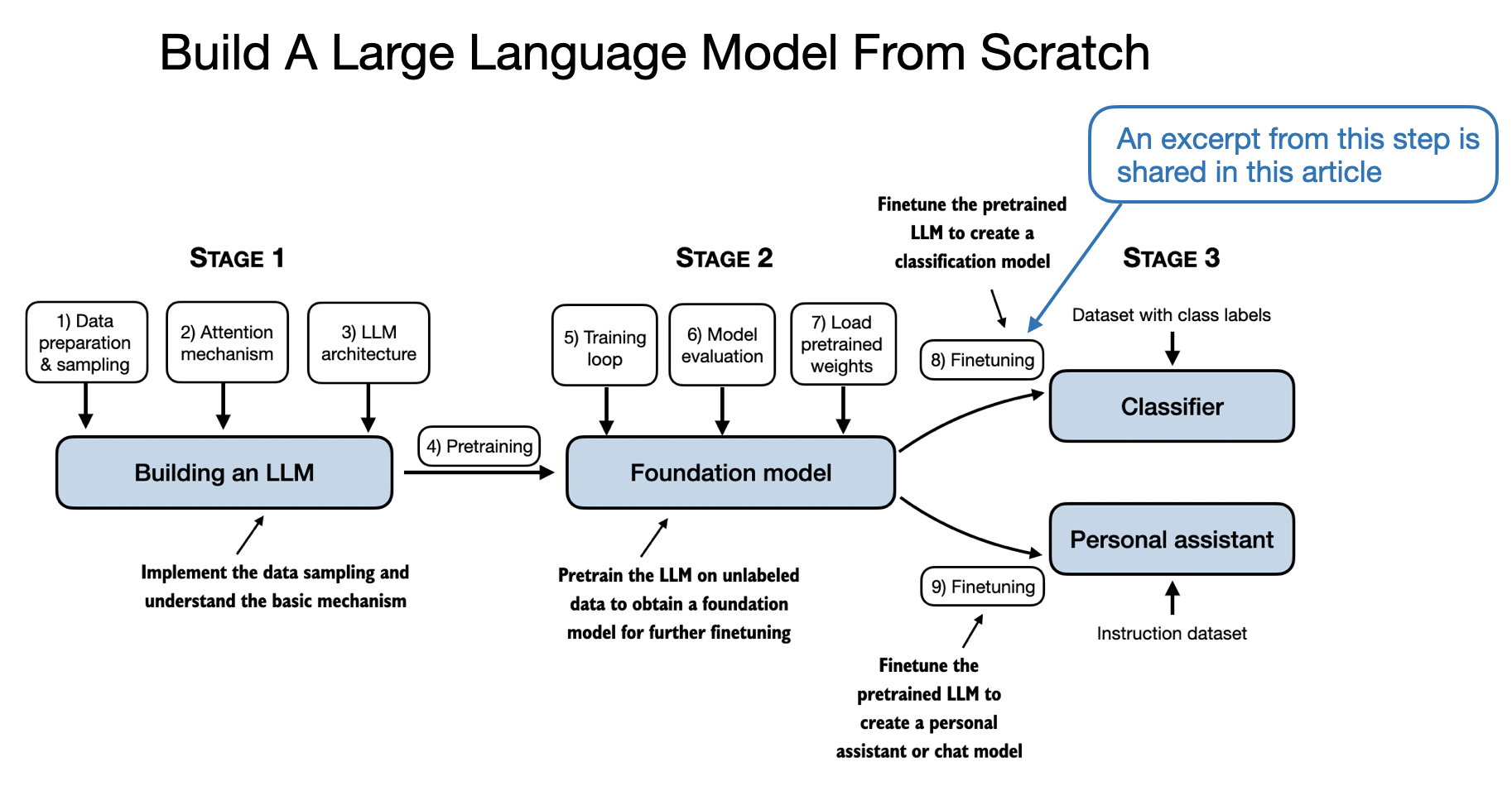
To provide some context on which part of the chapter this excerpt is focused on, this excerpt centers on the modification required to transform a general pretrained LLM into a specialized LLM for classification tasks, as shown in Figure 3 below.

But before we jump to the modification of the LLM mentioned in Figure 3 above, let’s have a brief look at the pretrained LLM we are working with.

So, for simplicity, as assume that we set up the code to load the model as follows:

model = GPTModel(BASE_CONFIG)
load_weights_into_gpt(model, params)
model.eval()

After loading the model weights into the GPTModel, we use the text generation utility function from the previous chapters to ensure that the model generates coherent text:

from chapter04 import generate_text_simple
from chapter05 import text_to_token_ids, token_ids_to_text

text_1 = "Every effort moves you"

token_ids = generate_text_simple(
    model=model,
    idx=text_to_token_ids(text_1, tokenizer),
    max_new_tokens=15,
    context_size=BASE_CONFIG["context_length"]
)

print(token_ids_to_text(token_ids, tokenizer))

As we can see based on the following output, the model generates coherent text, which is an indicator that the model weights have been loaded correctly:

Every effort moves you forward.
The first step is to understand the importance of your work

Now, before we start finetuning the model as a spam classifier, let’s see if the model can perhaps already classify spam messages by by prompting it with instructions:

text_2 = (
    "Is the following text 'spam'? Answer with 'yes' or 'no':"
    " 'You are a winner you have been specially"
    " selected to receive $1000 cash or a $2000 award.'"
)

token_ids = generate_text_simple(
    model=model,
    idx=text_to_token_ids(text_2, tokenizer),
    max_new_tokens=23,
    context_size=BASE_CONFIG["context_length"]
)

print(token_ids_to_text(token_ids, tokenizer))

The model output is as follows:

Is the following text 'spam'? Answer with 'yes' or 'no': 'You are a winner you have been specially selected to receive $1000 cash or a $2000 award.'
The following text 'spam'? Answer with 'yes' or 'no': 'You are a winner

Based on the output, it’s apparent that the model struggles with following instructions.

This is anticipated, as it has undergone only pretraining and lacks instruction finetuning, which we will explore in the upcoming chapter.

The next section prepares the model for classification finetuning.

Adding a classification head

In this section, we modify the pretrained large language model to prepare it for classification finetuning. To do this, we replace the original output layer, which maps the hidden representation to a vocabulary of 50,257 unique tokens, with a smaller output layer that maps to two classes: 0 (“not spam”) and 1 (“spam”), as shown in Figure 4 below.

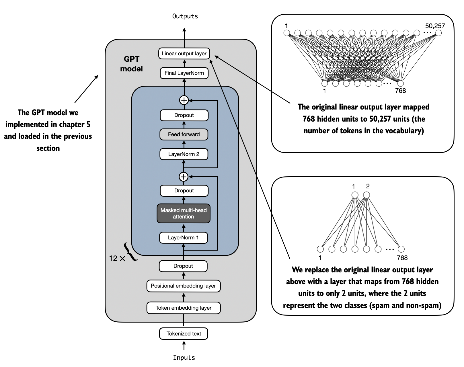
As shown in Figure 4 above, we use the same model as in previous chapters except for replacing the output layer.

Output layer nodes We could technically use a single output node since we are dealing with a binary classification task. However, this would require modifying the loss function, as discussed in an article in the Reference section in Appendix B. Therefore, we choose a more general approach where the number of output nodes matches the number of classes. For example, for a 3-class problem, such as classifying news articles as “Technology”, “Sports”, or “Politics”, we would use three output nodes, and so forth.*

Before we attempt the modification illustrated in Figure 4, let’s print the model architecture via print(model), which outputs the following:

GPTModel(
  (tok_emb): Embedding(50257, 768)
  (pos_emb): Embedding(1024, 768)
  (drop_emb): Dropout(p=0.0, inplace=False)
  (trf_blocks): Sequential(
...
    (11): TransformerBlock(
      (att): MultiHeadAttention(
        (W_query): Linear(in_features=768, out_features=768, bias=True)
        (W_key): Linear(in_features=768, out_features=768, bias=True)
        (W_value): Linear(in_features=768, out_features=768, bias=True)
        (out_proj): Linear(in_features=768, out_features=768, bias=True)
        (dropout): Dropout(p=0.0, inplace=False)
      )
      (ff): FeedForward(
        (layers): Sequential(
          (0): Linear(in_features=768, out_features=3072, bias=True)
          (1): GELU()
          (2): Linear(in_features=3072, out_features=768, bias=True)
        )
      )
      (norm1): LayerNorm()
      (norm2): LayerNorm()
      (drop_resid): Dropout(p=0.0, inplace=False)
    )
  )
  (final_norm): LayerNorm()
  (out_head): Linear(in_features=768, out_features=50257, bias=False)
)

Above, we can see the architecture we implemented in Chapter 4 neatly laid out. As discussed in Chapter 4, the GPTModel consists of embedding layers followed by 12 identical transformer blocks (only the last block is shown for brevity), followed by a final LayerNorm and the output layer, out_head.

Next, we replace the out_head with a new output layer, as illustrated in Figure 4, that we will finetune.

Finetuning selected layers versus all layers. Since we start with a pretrained model, it’s not necessary to finetune all model layers. This is because, in neural network-based language models, the lower layers generally capture basic language structures and semantics that are applicable across a wide range of tasks and datasets. So, finetuning only the last layers (layers near the output), which are more specific to nuanced linguistic patterns and task-specific features, can often be sufficient to adapt the model to new tasks. A nice side effect is that it is computationally more efficient to finetune only a small number of layers. Interested readers can find more information, including experiments, on which layers to finetune in the References section for this chapter in Appendix B.

To get the model ready for classification finetuning, we first freeze the model, meaning that we make all layers non-trainable:

for param in model.parameters():
    param.requires_grad = False

Then, as shown in Figure 4 earlier, we replace the output layer (model.out_head), which originally maps the layer inputs to 50,257 dimensions (the size of the vocabulary):

torch.manual_seed(123)

num_classes = 2

model.out_head = torch.nn.Linear(
    in_features=BASE_CONFIG["emb_dim"],
    out_features=num_classes
)

Note that in the preceding code, we use BASE_CONFIG["emb_dim"], which is equal to 768 in the "gpt2-small (124M)" model, to keep the code below more general. This means we can also use the same code to work with the larger GPT-2 model variants.

This new model.out_head output layer has its requires_grad attribute set to True by default, which means that it’s the only layer in the model that will be updated during training.

Technically, training the output layer we just added is sufficient. However, as I found in experiments, finetuning additional layers can noticeably improve the predictive performance of the finetuned model. (For more details, refer to the References in Appendix C.)

Additionally, we configure the last transformer block and the final LayerNorm module, which connects this block to the output layer, to be trainable, as depicted in Figure 5 below.

To make the final LayerNorm and last transformer block trainable, as illustrated in Figure 5 above, we set their respective requires_grad to True:

for param in model.trf_blocks[-1].parameters():
    param.requires_grad = True

for param in model.final_norm.parameters():
    param.requires_grad = True

Even though we added a new output layer and marked certain layers as trainable or non-trainable, we can still use this model in a similar way to previous chapters. For instance, we can feed it an example text identical to how we have done it in earlier chapters. For example, consider the following example text:

inputs = tokenizer.encode("Do you have time")
inputs = torch.tensor(inputs).unsqueeze(0)

print("Inputs:", inputs)
print("Inputs dimensions:", inputs.shape)

As the print output shows, the preceding code encodes the inputs into a tensor consisting of 4 input tokens:

Inputs: tensor([[5211,  345,  423,  640]])
Inputs dimensions: torch.Size([1, 4])

Then, we can pass the encoded token IDs to the model as usual:

with torch.no_grad():
    outputs = model(inputs)

print("Outputs:\n", outputs)
print("Outputs dimensions:", outputs.shape)

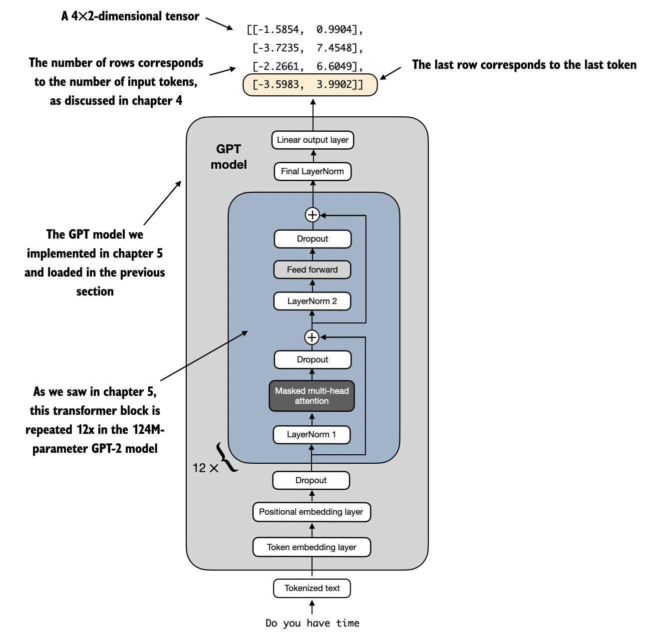
The output tensor looks like as follows:

Outputs:
 tensor([[[-1.5854,  0.9904],
          [-3.7235,  7.4548],
          [-2.2661,  6.6049],
          [-3.5983,  3.9902]]])
Outputs dimensions: torch.Size([1, 4, 2])

In Chapters 4 and 5, a similar input would have produced an output tensor of shape [1, 4, 50257], where 50,257 represents the vocabulary size. As in previous chapters, the number of output rows corresponds to the number of input tokens (in this case, 4). However, each output’s embedding dimension (the number of columns) is now reduced to 2 instead of 50,257 since we replaced the output layer of the model.

Remember that we are interested in finetuning this model so that it returns a class label that indicates whether a model input is spam or not spam. To achieve this, we don’t need to finetune all 4 output rows but can focus on a single output token. In particular, we will focus on the last row corresponding to the last output token, as illustrated in Figure 6 below.

To extract the last output token, illustrated in Figure 6 above, from the output tensor, we use the following code:

print("Last output token:", outputs[:, -1, :])

This prints the following:

Last output token: tensor([[-3.5983,  3.9902]])

Before we proceed to the next section, let’s recap our discussion. We will focus on converting the values into a class label prediction. But first, let’s understand why we are particularly interested in the last output token, and not the 1st, 2nd, or 3rd output token.

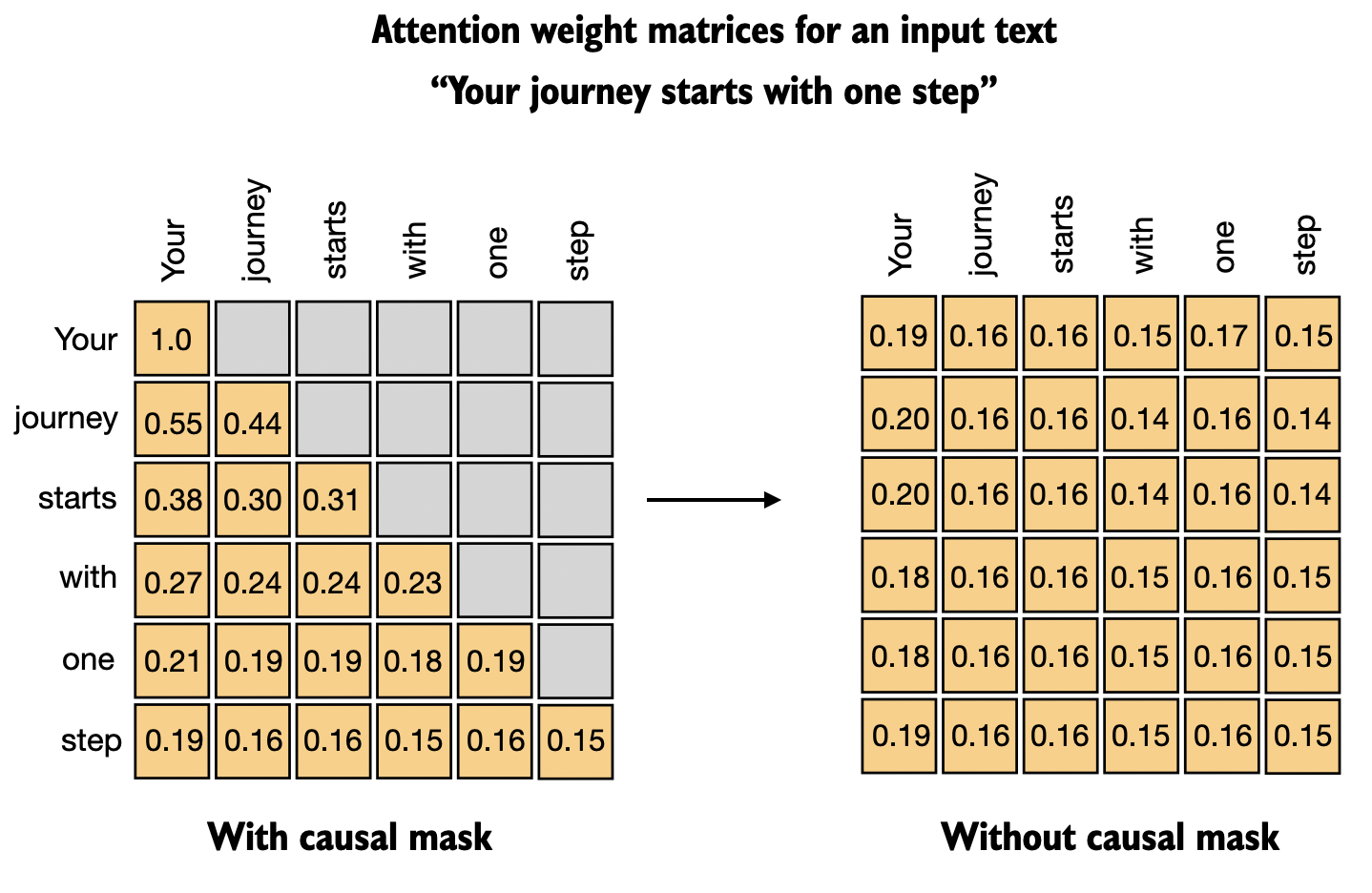
In Chapter 3, we explored the attention mechanism, which establishes a relationship between each input token and every other input token. Subsequently, we introduced the concept of a causal attention mask, commonly used in GPT-like models. This mask restricts a token’s focus to only its current position and those before it, ensuring that each token can only be influenced by itself and preceding tokens, as illustrated in Figure 7 below.

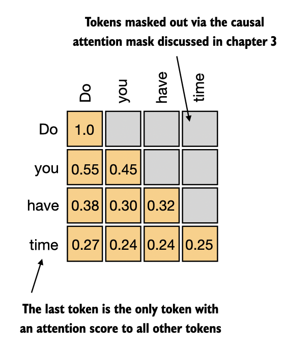
Given the causal attention mask setup shown in Figure 7 above, the last token in a sequence accumulates the most information since it is the only token with access to data from all the previous tokens. Therefore, in our spam classification task, we focus on this last token during the finetuning process.

Having modified the model, the next section will detail the process of transforming the last token into class label predictions and calculate the model’s initial prediction accuracy. Following this, we will finetune the model for the spam classification task in the subsequent section.

Evaluating the model performance

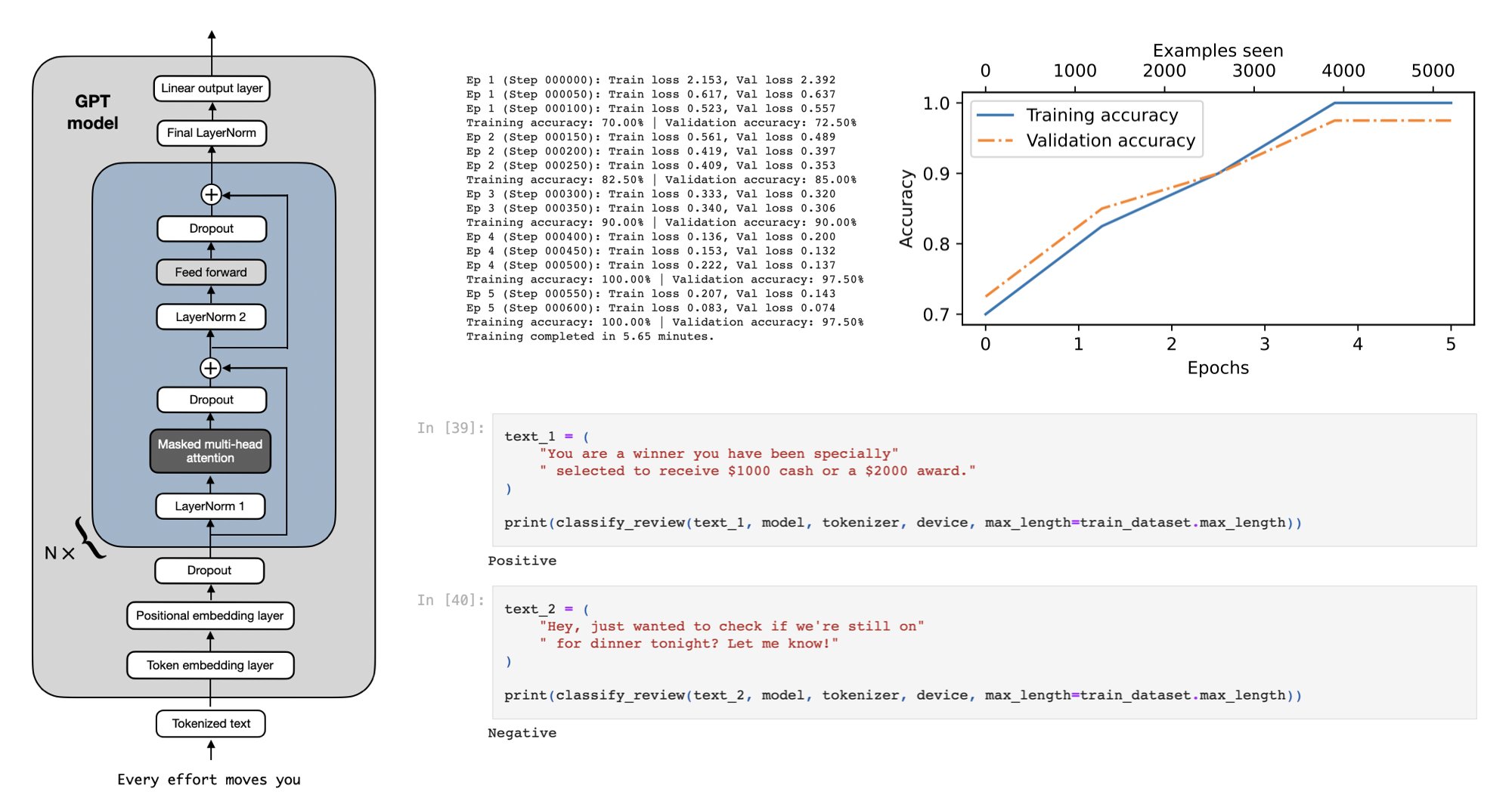
Since this excerpt was already long, I won’t go into the details on the model evaluation. However, I wanted to share at least the plot showing the classification accuracy on the training and validation sets during training to show you that the model indeed learns really well.

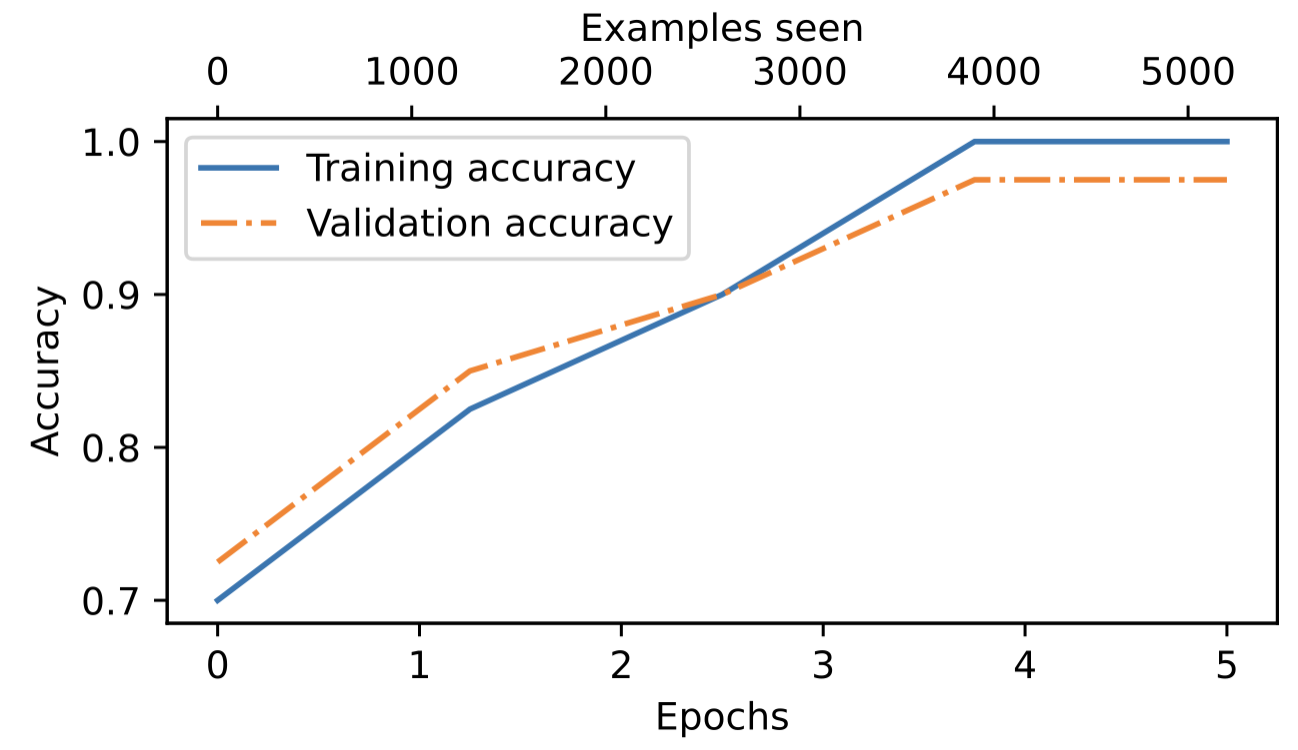
As we can see in Figure 8 above, the model achieves a validation accuracy of approximately 97%. The test accuracy (not shown) is approximately 96%. Furthermore, we can see that the model slightly overfits, as indicated by the slightly higher training set accuracy. Overall, though, this model performed really well: a 96% test set accuracy means that it correctly identifies 96 out of 100 messages as spam or not spam. (We didn’t discuss the dataset in this excerpt, but it was a balanced dataset with 50% spam and 50% non-spam messages, which means that a random or badly trained classifier would achieve approximately 50% classification accuracy.)

Insights from additional experiments

You may have many questions about certain design choices at this point, so I wanted to share a few results from some additional experiments I ran, which may address one or more questions or concerns you might have. The code to reproduce these experiments is available here on GitHub.

Disclaimer: the experiments were mostly only run on 1 dataset, and should be repeated on other datasets in the future to test whether these findings generalize.

1) Do we need to train all layers?

In the chapter excerpt above, we only trained the output layer and the last transformer block for efficiency reasons. As explained earlier, for classification finetuning, it is not necessary to update all layers in an LLM. (The fewer weights we update, the faster the training will be because we don’t need to compute the gradients for these weights during backpropagation.)

However, you may wonder how much predictive performance we are leaving on the table by not updating all layers. So, in the table below, I ran a comparison between finetuning all layers, only the last transformer block (plus the last layer), and the last layer only.

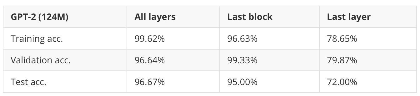
As shown in Table 1 above, training all layers results in a slightly better performance: 96.67% versus 95.00%. (This increased the runtime by about 2.5fold, though.)

The complete set of experiments can be found here on GitHub.

2) Why finetuning the last token, not the first token?

If you are familiar with encoder-style language models like BERT (BERT: Pre-training of Deep Bidirectional Transformers for Language Understanding” by Devlin et al. 2018), you may know that these have a designated classification token as their first token, as shown in the figure below.

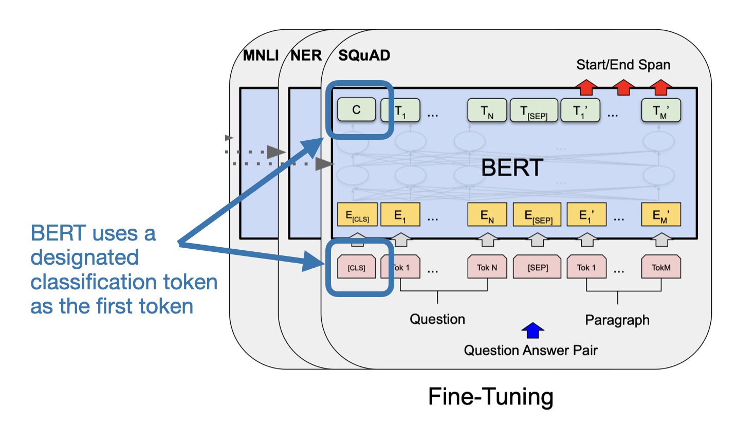
In contrast to BERT, GPT is a decoder-style model with a causal attention mask (shown in Figure 7 earlier). This means the first token has no context information of any other token in the input. Only the last token has information about all other tokens.

Hence, if we want to use models like GPT for classification finetuning, we should focus on the last token to capture contextual information of all other input tokens.

Below is additional experimental evidence, where we can see that using the first token to finetune a GPT model for classification results in a much worse performance.

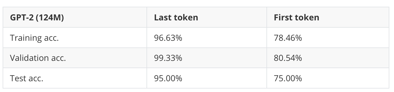
Overall, I find it still surprising, though, that the first token contains so much information to determine whether a message is spam or not with 75% accuracy. (Not that this is a balanced dataset, and a random classifier yields 50% accuracy).

3) How does BERT compare to GPT performance-wise?

Speaking of BERT, you may wonder how it compares to a GPT-style model on classification tasks.

In short, the small GPT-2 model from the previous section and BERT performed similarly well on the spam classification dataset, as shown in the table below.

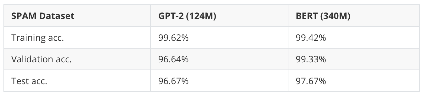
Note that the BERT model performs slightly better (1% higher test accuracy), but it is also almost 3x larger. Furthermore, the dataset may be too small and simple, so I also tried the IMDB Movie Review dataset for sentiment classification (that is, predicting whether a reviewer liked the movie or not).

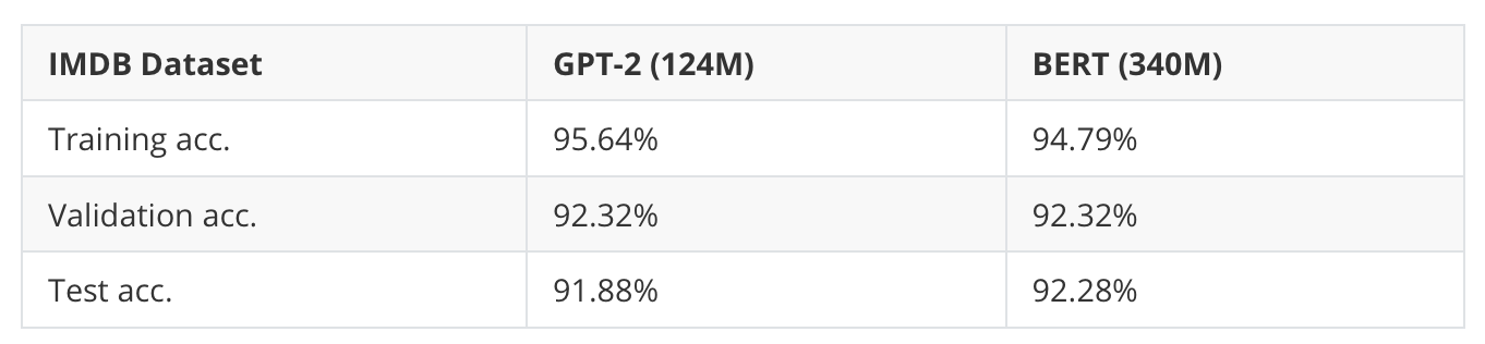
As we can see, the two models, GPT-2 and BERT, also have relatively similar predictive performances on this larger dataset (consisting of 25k training and 25k test set records).

Generally, BERT and other encoder-style models were considered superior to decoder-style models for classification tasks. However, as the experiments above showed, there’s not a large difference between the encoder-style BERT and the decoder-style GPT model.

Furthermore, if you are interested in more benchmark comparison and tips for improving decoder-style models for classification further, you might like these two recent papers:

• Label Supervised LLaMA Finetuning (2023) by Li et al.
• LLM2Vec: Large Language Models Are Secretly Powerful Text Encoders (2024) by BehnamGhader et al.

For instance, as the papers above discuss, one can improve the classification performance of decoder-style models further by removing the causal mask during classification finetuning.

4) Should we disable the causal mask?

Since we train GPT-like models on a next-word prediction task, a core feature of the GPT architecture is the causal attention mask (different from BERT models or the original transformer architecture).

However, we could actually remove the causal mask during classification finetuning, which would allow us to finetune the first rather than the last token since future tokens will no longer be masked, and the first token can see all other tokens.

Disabling a causal attention mask in a GPT-like LLM fortunately requires changing only 2 lines of code:

class MultiheadAttention(nn.Module):
    def __init__(self, d_in, d_out, context_length, dropout, num_heads):
        super().__init__()
        # ...

    def forward(self, x):
        b, num_tokens, d_in = x.shape
        keys = self.W_key(x)  # Shape: (b, num_tokens, d_out)
        queries = self.W_query(x)
        values = self.W_value(x)

        # ...

        attn_scores = queries @ keys.transpose(2, 3)

        # Comment out the causal attention mask part
        # mask_bool = self.mask.bool()[:num_tokens, :num_tokens]
        # attn_scores.masked_fill_(mask_bool, -torch.inf)

        attn_weights = torch.softmax(
             attn_scores / keys.shape[-1]**0.5, dim=-1
        )
        context_vec = (attn_weights @ values).transpose(1, 2)
        context_vec = context_vec.contiguous().view(
            b, num_tokens, self.d_out
        )
        context_vec = self.out_proj(context_vec)
        return context_vec

Table 5 below shows how this modification affects the performance of the spam classification task.

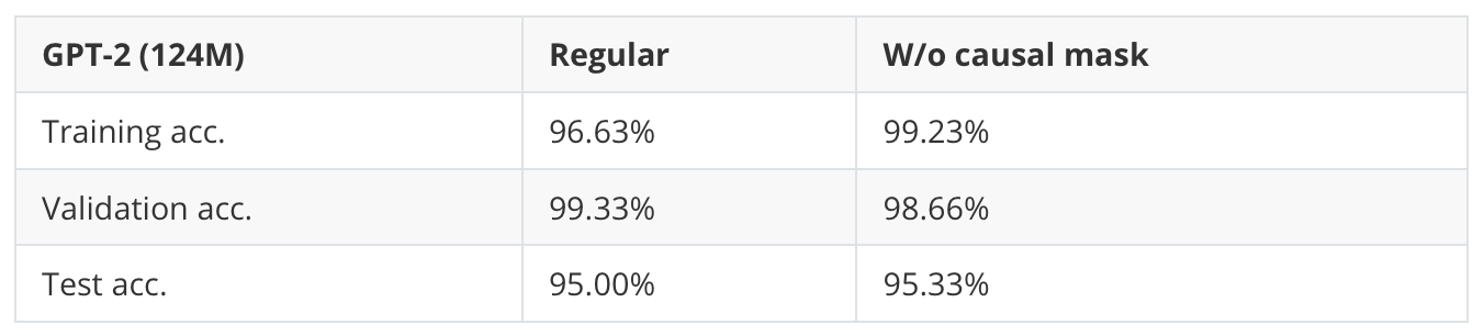
As we can see based on the results in Table 5, we can get a small improvement when we disable the causal mask during finetuning.

5) What impact does increasing the model size have?

So far, we’ve only looked at the performance of the smallest GPT-2 model, the 124 million-parameter version. How does it compare to the larger variants, which have 355 million, 774 million, and 1.5 billion parameters. The results are summarized in Table 6.

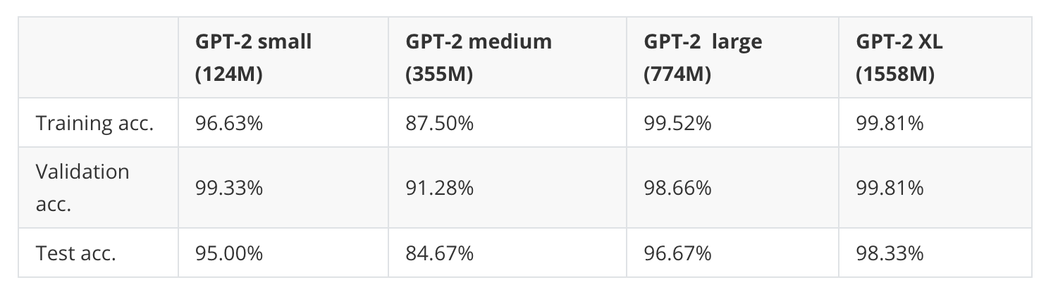
As we can see, the the prediction accuracy improves significantly with larger models (however, GPT-2 medium is an outlier here. I have noticed poor performance of this model on other datasets, too, and I suspect that the model has potentially not been pretrained very well.)

However, while the GPT-2 XL model shows a noticeably better classification accuracy than the smallest model, it also took 7x longer to finetune.

6) What improvements can we expect from LoRA?

In the very first question, “1) Do we need to train all layers?” we found that we could (almost) match the classification performance when finetuning only the last transformer block instead of finetuning the whole model. The advantage of only finetuning the last block is that the training is faster since not all weight parameters are being updated.

A follow-up question is how this compares to Low-Rank Adaptation (LoRA), a parameter-efficient finetuning technique. (LoRA is covered in Appendix E.)

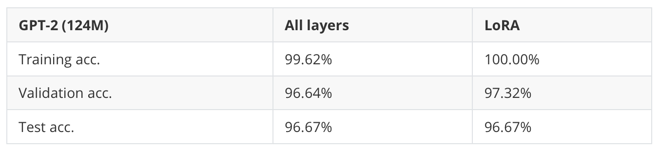
As we can see in Table 7 above, both full finetuning (all layers) and LoRA result in the same test set performance on this dataset.

On the small model, LoRA is slightly slower since the additional overhead from adding LoRA layers may outweigh the benefits, but when training the larger 1.5 billion parameters model, LoRA trains 1.53x faster.

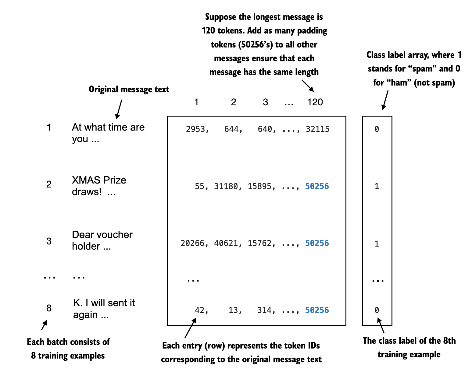
7) Padding or no padding?

If we want to process data in batches during training or inference (this involves processing more than one input sequence at a time), we need to insert padding tokens to ensure that the training examples are of equal length.

In regular text generation tasks, padding doesn’t affect the model response since padding tokens are usually added to the right side, and due to the causal mask discussed earlier, these padding tokens don’t influence the other tokens.

However, remember that we finetuned the last token, as discussed earlier. Since the padding tokens are to the left of this last token, the padding tokens may affect the result.

If we use a batch size of 1, we actually don’t need to pad the inputs. This is, of course, more inefficient from a computational standpoint (since we only process one input example at a time). Still, a batch size of 1 can be used as a workaround to test whether or not using padding can improve the results. (An alternative solution is to add a custom mask to ignore padding tokens in the attention score computation, but since this would require changing the GPT implementation, that’s a topic for another time.)

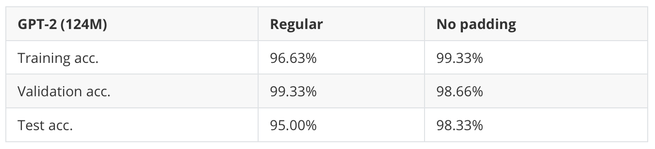
As we can see, avoiding padding tokens can indeed give the model a noticeable boost! (Note that I used gradient accumulation to simulate a batch size of 8 to match the batch size of the default experiment and make it a fair comparison.)

I hope you found these additional experiments interesting. I have a few more as bonus material here on GitHub.

Build A Large Language Model From Scratch

This article presents a 10-page snippet from Chapter 6 of my new book, “Build a Large Language Model from Scratch.”

What you’ve read is just a small part of the entire 365-page journey of building a GPT-like LLM from scratch to understand how LLMs really work.

If this excerpt resonated with you, you might find the rest of the book equally insightful and helpful.

• Manning link
• Amazon link (preorder)

Your support means a great deal and is tremendously helpful in continuing this journey. Thank you!