Understanding and Coding the Self-Attention Mechanism of Large Language Models From Scratch
In this article, we are going to understand how self-attention works from scratch. This means we will code it ourselves one step at a time.
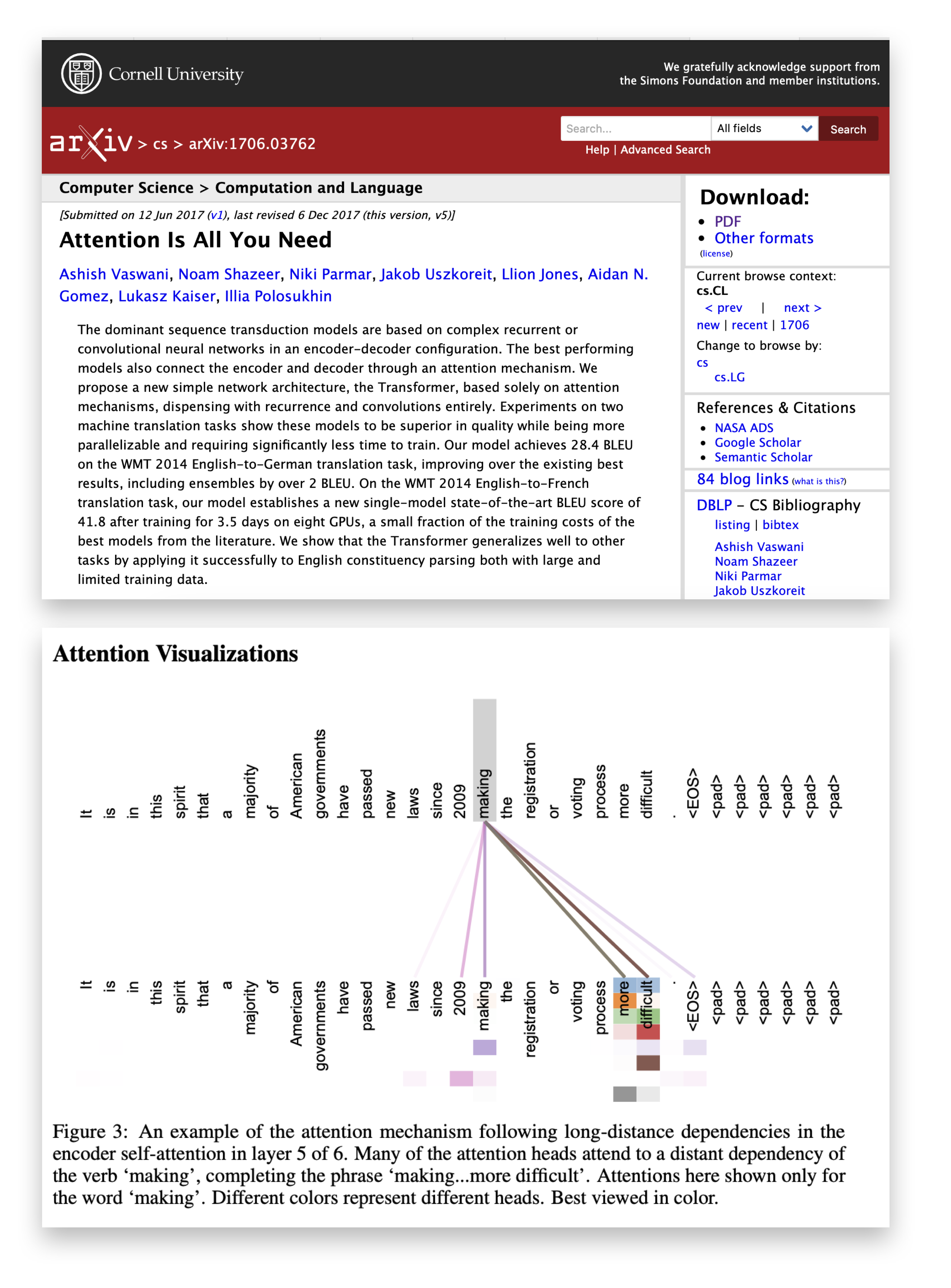
Since its introduction via the original transformer paper (Attention Is All You Need), self-attention has become a cornerstone of many state-of-the-art deep learning models, particularly in the field of Natural Language Processing (NLP). Since self-attention is now everywhere, it’s important to understand how it works.
Self-Attention
The concept of “attention” in deep learning has its roots in the effort to improve Recurrent Neural Networks (RNNs) for handling longer sequences or sentences. For instance, consider translating a sentence from one language to another. Translating a sentence word-by-word does not work effectively.
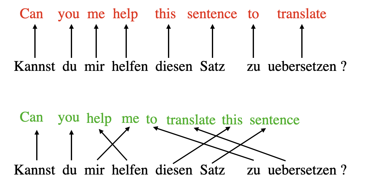
To overcome this issue, attention mechanisms were introduced to give access to all sequence elements at each time step. The key is to be selective and determine which words are most important in a specific context. In 2017, the transformer architecture introduced a standalone self-attention mechanism, eliminating the need for RNNs altogether.
(For brevity, and to keep the article focused on the technical self-attention details, and I am skipping parts of the motivation, but my Machine Learning with PyTorch and Scikit-Learn book has some additional details in Chapter 16 if you are interested.)
We can think of self-attention as a mechanism that enhances the information content of an input embedding by including information about the input’s context. In other words, the self-attention mechanism enables the model to weigh the importance of different elements in an input sequence and dynamically adjust their influence on the output. This is especially important for language processing tasks, where the meaning of a word can change based on its context within a sentence or document.
Note that there are many variants of self-attention. A particular focus has been on making self-attention more efficient. However, most papers still implement the original scaled-dot product attention mechanism discussed in this paper since it usually results in superior accuracy and because self-attention is rarely a computational bottleneck for most companies training large-scale transformers.
In this article, we focus on the original scaled-dot product attention mechanism (referred to as self-attention), which remains the most popular and most widely used attention mechanism in practice. However, if you are interested in other types of attention mechanisms, check out the 2020 Efficient Transformers: A Survey and the 2023 A Survey on Efficient Training of Transformers review and the recent FlashAttention paper.
Embedding an Input Sentence
Before we begin, let’s consider an input sentence “Life is short, eat dessert first” that we want to put through the self-attention mechanism. Similar to other types of modeling approaches for processing text (e.g., using recurrent neural networks or convolutional neural networks), we create a sentence embedding first.
For simplicity, here our dictionary dc is restricted to the words that occur in the input sentence. In a real-world application, we would consider all words in the training dataset (typical vocabulary sizes range between 30k to 50k).
In:
sentence = 'Life is short, eat dessert first'

dc = {s:i for i,s in enumerate(sorted(sentence.replace(',', '').split()))}
print(dc)
Out:
{'Life': 0, 'dessert': 1, 'eat': 2, 'first': 3, 'is': 4, 'short': 5}
Next, we use this dictionary to assign an integer index to each word:
In:
import torch

sentence_int = torch.tensor([dc[s] for s in sentence.replace(',', '').split()])
print(sentence_int)
Out:
tensor([0, 4, 5, 2, 1, 3])
Now, using the integer-vector representation of the input sentence, we can use an embedding layer to encode the inputs into a real-vector embedding. Here, we will use a 16-dimensional embedding such that each input word is represented by a 16-dimensional vector. Since the sentence consists of 6 words, this will result in a \(6 \times 16\)-dimensional embedding:
In:
torch.manual_seed(123)
embed = torch.nn.Embedding(6, 16)
embedded_sentence = embed(sentence_int).detach()

print(embedded_sentence)
print(embedded_sentence.shape)
Out:
tensor([[ 0.3374, -0.1778, -0.3035, -0.5880,  0.3486,  0.6603, -0.2196, -0.3792,
          0.7671, -1.1925,  0.6984, -1.4097,  0.1794,  1.8951,  0.4954,  0.2692],
        [ 0.5146,  0.9938, -0.2587, -1.0826, -0.0444,  1.6236, -2.3229,  1.0878,
          0.6716,  0.6933, -0.9487, -0.0765, -0.1526,  0.1167,  0.4403, -1.4465],
        [ 0.2553, -0.5496,  1.0042,  0.8272, -0.3948,  0.4892, -0.2168, -1.7472,
         -1.6025, -1.0764,  0.9031, -0.7218, -0.5951, -0.7112,  0.6230, -1.3729],
        [-1.3250,  0.1784, -2.1338,  1.0524, -0.3885, -0.9343, -0.4991, -1.0867,
          0.8805,  1.5542,  0.6266, -0.1755,  0.0983, -0.0935,  0.2662, -0.5850],
        [-0.0770, -1.0205, -0.1690,  0.9178,  1.5810,  1.3010,  1.2753, -0.2010,
          0.4965, -1.5723,  0.9666, -1.1481, -1.1589,  0.3255, -0.6315, -2.8400],
        [ 0.8768,  1.6221, -1.4779,  1.1331, -1.2203,  1.3139,  1.0533,  0.1388,
          2.2473, -0.8036, -0.2808,  0.7697, -0.6596, -0.7979,  0.1838,  0.2293]])
torch.Size([6, 16])
Defining the Weight Matrices
Now, let’s discuss the widely utilized self-attention mechanism known as the scaled dot-product attention, which is integrated into the transformer architecture.
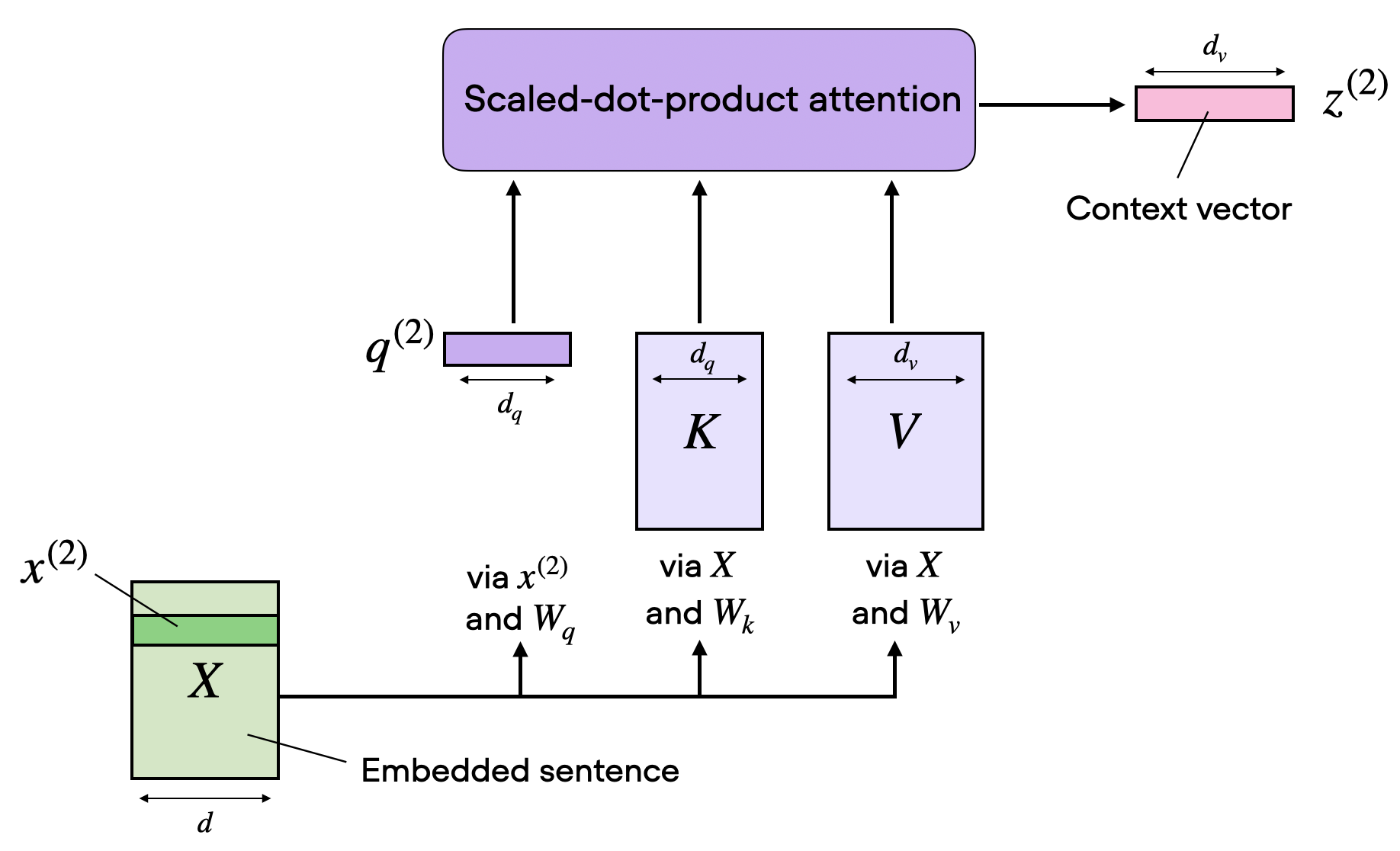
Self-attention utilizes three weight matrices, referred to as \(\mathbf{W}_q\), \(\mathbf{W}_k\), and \(\mathbf{W}_v\), which are adjusted as model parameters during training. These matrices serve to project the inputs into query, key, and value components of the sequence, respectively.
The respective query, key and value sequences are obtained via matrix multiplication between the weight matrices \(\mathbf{W}\) and the embedded inputs \(\mathbf{x}\):
- Query sequence: \(\mathbf{q}^{(i)}=\mathbf{W}_q \mathbf{x}^{(i)}\) for \(i \in[1, T]\)
- Key sequence: \(\mathbf{k}^{(i)}=\mathbf{W}_k \mathbf{x}^{(i)}\) for \(i \in[1, T]\)
- Value sequence: \(\mathbf{v}^{(i)}=\mathbf{W}_v \mathbf{x}^{(i)}\) for \(i \in[1, T]\)
The index \(i\) refers to the token index position in the input sequence, which has length \(T\).
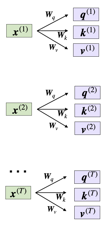
Here, both \(\mathbf{q}^{(i)}\) and \(\mathbf{k}^{(i)}\) are vectors of dimension \(d_k\). The projection matrices \(\mathbf{W}_{q}\) and \(\mathbf{W}_{k}\) have a shape of \(d_k \times d\), while \(\mathbf{W}_{v}\) has the shape \(d_v \times d\).
(It’s important to note that \(d\) represents the size of each word vector, \(\mathbf{x}\).)
Since we are computing the dot-product between the query and key vectors, these two vectors have to contain the same number of elements (\(d_q = d_k\)). However, the number of elements in the value vector \(\mathbf{v}^{(i)}\), which determines the size of the resulting context vector, is arbitrary.
So, for the following code walkthrough, we will set \(d_q = d_k = 24\) and use \(d_v = 28\), initializing the projection matrices as follows:
In:
torch.manual_seed(123)

d = embedded_sentence.shape[1]

d_q, d_k, d_v = 24, 24, 28

W_query = torch.nn.Parameter(torch.rand(d_q, d))
W_key = torch.nn.Parameter(torch.rand(d_k, d))
W_value = torch.nn.Parameter(torch.rand(d_v, d))
Computing the Unnormalized Attention Weights
Now, let’s suppose we are interested in computing the attention-vector for the second input element – the second input element acts as the query here:
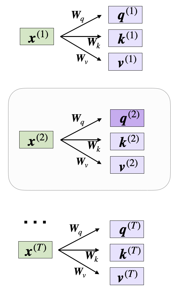
In code, this looks like as follows:
In:
x_2 = embedded_sentence[1]
query_2 = W_query.matmul(x_2)
key_2 = W_key.matmul(x_2)
value_2 = W_value.matmul(x_2)

print(query_2.shape)
print(key_2.shape)
print(value_2.shape)
torch.Size([24])
torch.Size([24])
torch.Size([28])
We can then generalize this to compute th remaining key, and value elements for all inputs as well, since we will need them in the next step when we compute the unnormalized attention weights \(\omega\):
In:
keys = W_key.matmul(embedded_sentence.T).T
values = W_value.matmul(embedded_sentence.T).T

print("keys.shape:", keys.shape)
print("values.shape:", values.shape)
Out:
keys.shape: torch.Size([6, 24])
values.shape: torch.Size([6, 28])
Now that we have all the required keys and values, we can proceed to the next step and compute the unnormalized attention weights \(\omega\) , which are illustrated in the figure below:
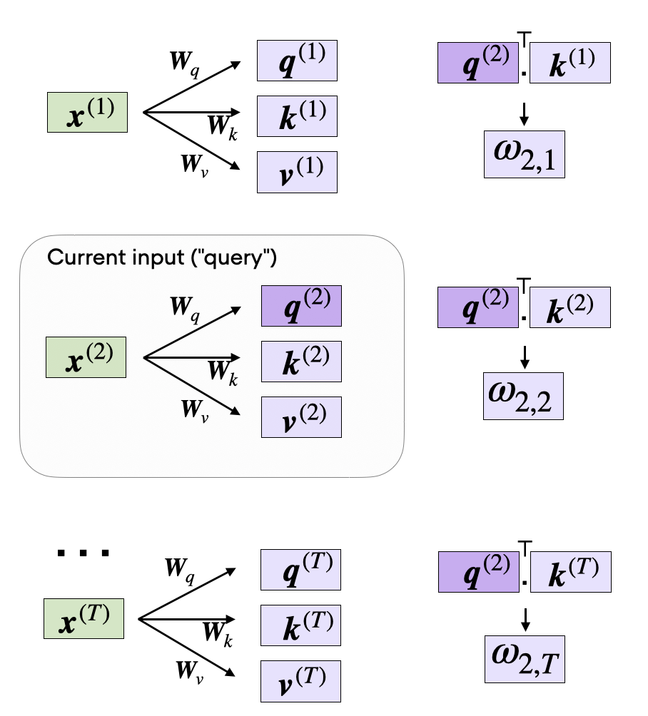
As illustrated in the figure above, we compute \(\omega_{i, j}\) as the dot product between the query and key sequences, \(\omega_{i j}=\mathbf{q}^{(i)^{\top}} \mathbf{k}^{(j)}\).
For example, we can compute the unnormalized attention weight for the query and 5th input element (corresponding to index position 4) as follows:
In:
omega_24 = query_2.dot(keys[4])
print(omega_24)
Out:
tensor(11.1466)
Since we will need those to compute the attention scores later, let’s compute the \(\omega\) values for all input tokens as illustrated in the previous figure:
In:
omega_2 = query_2.matmul(keys.T)
print(omega_2)
Out:
tensor([ 8.5808, -7.6597, 3.2558, 1.0395, 11.1466, -0.4800])
Computing the Attention Scores
The subsequent step in self-attention is to normalize the unnormalized attention weights, \(\omega\), to obtain the normalized attention weights, \(\alpha\), by applying the softmax function. Additionally, \(1/\sqrt{d_k}\) is used to scale \(\omega\) before normalizing it through the softmax function, as shown below:
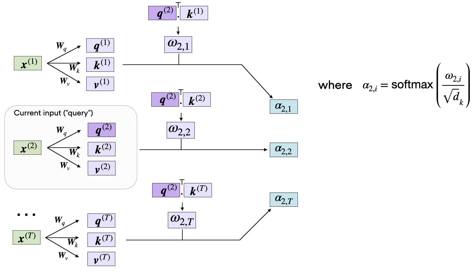
The scaling by the square-root of \(d_k\) ensures that the Euclidean length of the weight vectors will be approximately in the same magnitude. This helps prevent the attention weights from becoming too small or too large, which could lead to numerical instability or affect the model’s ability to converge during training.
Why does specifically \(\sqrt{d_k}\)? The dot product between q and k is a sum of \(d_k\) independent terms, each with variance about 1. That means the variance of the raw score grows linearly with \(d_k\). By dividing by \(\sqrt{d_k}\), we cancel that growth and bring the variance back to about 1.
In code, we can implement the computation of the attention weights as follows:
In:
import torch.nn.functional as F

attention_weights_2 = F.softmax(omega_2 / d_k**0.5, dim=0)
print(attention_weights_2)
Out:
tensor([0.2912, 0.0106, 0.0982, 0.0625, 0.4917, 0.0458])
Finally, the last step is to compute the context vector \(\mathbf{z}^{(2)}\), which is an attention-weighted version of our original query input \(\mathbf{x}^{(2)}\), including all the other input elements as its context via the attention weights:
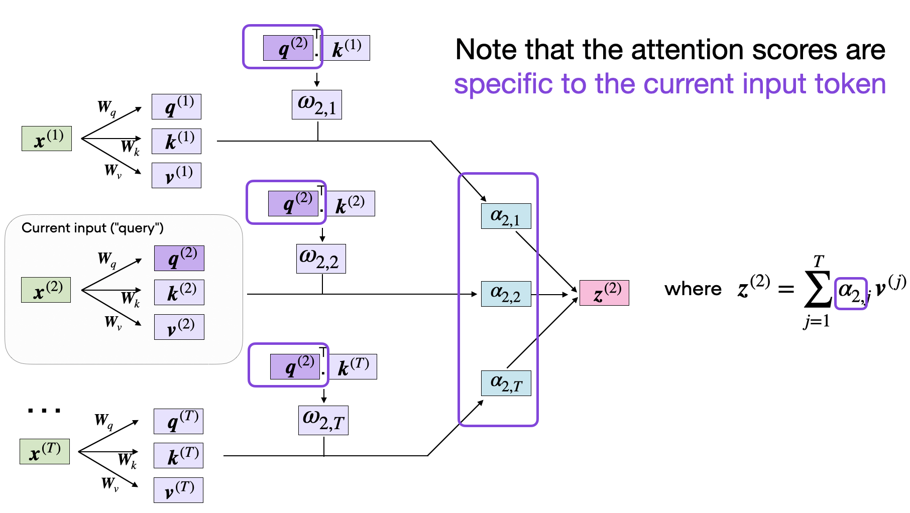
In code, this looks like as follows:
In:
context_vector_2 = attention_weights_2.matmul(values)

print(context_vector_2.shape)
print(context_vector_2)
Out:
torch.Size([28])
tensor(torch.Size([28])
tensor([-1.5993,  0.0156,  1.2670,  0.0032, -0.6460, -1.1407, -0.4908, -1.4632,
         0.4747,  1.1926,  0.4506, -0.7110,  0.0602,  0.7125, -0.1628, -2.0184,
         0.3838, -2.1188, -0.8136, -1.5694,  0.7934, -0.2911, -1.3640, -0.2366,
        -0.9564, -0.5265,  0.0624,  1.7084])
Note that this output vector has more dimensions (\(d_v=28\)) than the original input vector (\(d=16\)) since we specified \(d_v > d\) earlier; however, the embedding size choice is arbitrary.
Multi-Head Attention
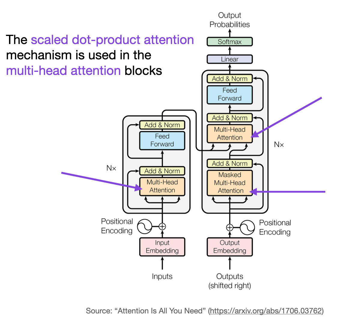
In the very first figure, at the top of this article, we saw that transformers use a module called multi-head attention. How does that relate to the self-attention mechanism (scaled-dot product attention) we walked through above?
In the scaled dot-product attention, the input sequence was transformed using three matrices representing the query, key, and value. These three matrices can be considered as a single attention head in the context of multi-head attention. The figure below summarizes this single attention head we covered previously:
As its name implies, multi-head attention involves multiple such heads, each consisting of query, key, and value matrices. This concept is similar to the use of multiple kernels in convolutional neural networks.
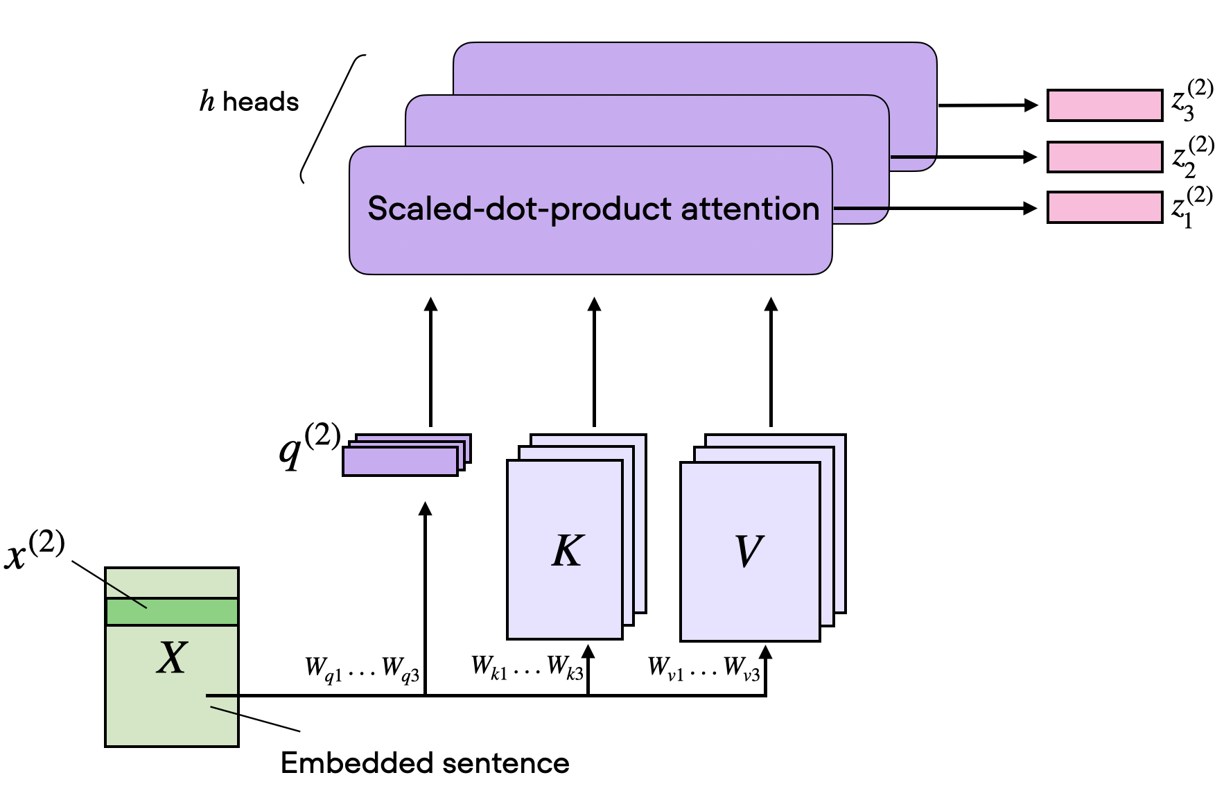
To illustrate this in code, suppose we have 3 attention heads, so we now extend the \(d' \times d\) dimensional weight matrices so \(3 \times d' \times d\):
In:
h = 3
multihead_W_query = torch.nn.Parameter(torch.rand(h, d_q, d))
multihead_W_key = torch.nn.Parameter(torch.rand(h, d_k, d))
multihead_W_value = torch.nn.Parameter(torch.rand(h, d_v, d))
Consequently, each query element is now \(3 \times d_q\) dimensional, where \(d_q=24\) (here, let’s keep the focus on the 3rd element corresponding to index position 2):
In:
multihead_query_2 = multihead_W_query.matmul(x_2)
print(multihead_query_2.shape)
Out:
torch.Size([3, 24])
We can then obtain the keys and values in a similar fashion:
In:
multihead_key_2 = multihead_W_key.matmul(x_2)
multihead_value_2 = multihead_W_value.matmul(x_2)
Now, these key and value elements are specific to the query element. But, similar to earlier, we will also need the value and keys for the other sequence elements in order to compute the attention scores for the query. We can do this is by expanding the input sequence embeddings to size 3, i.e., the number of attention heads:
In:
stacked_inputs = embedded_sentence.T.repeat(3, 1, 1)
print(stacked_inputs.shape)
Out:
torch.Size([3, 16, 6])
Now, we can compute all the keys and values using via torch.bmm() ( batch matrix multiplication):
In:
multihead_keys = torch.bmm(multihead_W_key, stacked_inputs)
multihead_values = torch.bmm(multihead_W_value, stacked_inputs)
print("multihead_keys.shape:", multihead_keys.shape)
print("multihead_values.shape:", multihead_values.shape)
Out:
multihead_keys.shape: torch.Size([3, 24, 6])
multihead_values.shape: torch.Size([3, 28, 6])
We now have tensors that represent the three attention heads in their first dimension. The third and second dimensions refer to the number of words and the embedding size, respectively. To make the values and keys more intuitive to interpret, we will swap the second and third dimensions, resulting in tensors with the same dimensional structure as the original input sequence, embedded_sentence:
In:
multihead_keys = multihead_keys.permute(0, 2, 1)
multihead_values = multihead_values.permute(0, 2, 1)
print("multihead_keys.shape:", multihead_keys.shape)
print("multihead_values.shape:", multihead_values.shape)
Out:
multihead_keys.shape: torch.Size([3, 6, 24])
multihead_values.shape: torch.Size([3, 6, 28])
Then, we follow the same steps as previously to compute the unscaled attention weights \(\omega\) and attention weights \(\alpha\), followed by the scaled-softmax computation to obtain an \(h \times d_v\) (here: \(3 \times d_v\)) dimensional context vector \(\mathbf{z}\) for the input element \(\mathbf{x}^{(2)}\).
Cross-Attention
In the code walkthrough above, we set \(d_q = d_k = 24\) and \(d_v=28\). Or in other words, we used the same dimensions for query and key sequences. While the value matrix \(\mathbf{W}_v\) is often chosen to have the same dimension as the query and key matrices (such as in PyTorch’s MultiHeadAttention class), we can select an arbitrary number size for the value dimensions.
Since the dimensions are sometimes a bit tricky to keep track of, let’s summarize everything we have covered so far in the figure below, which depicts the various tensor sizes for a single attention head.
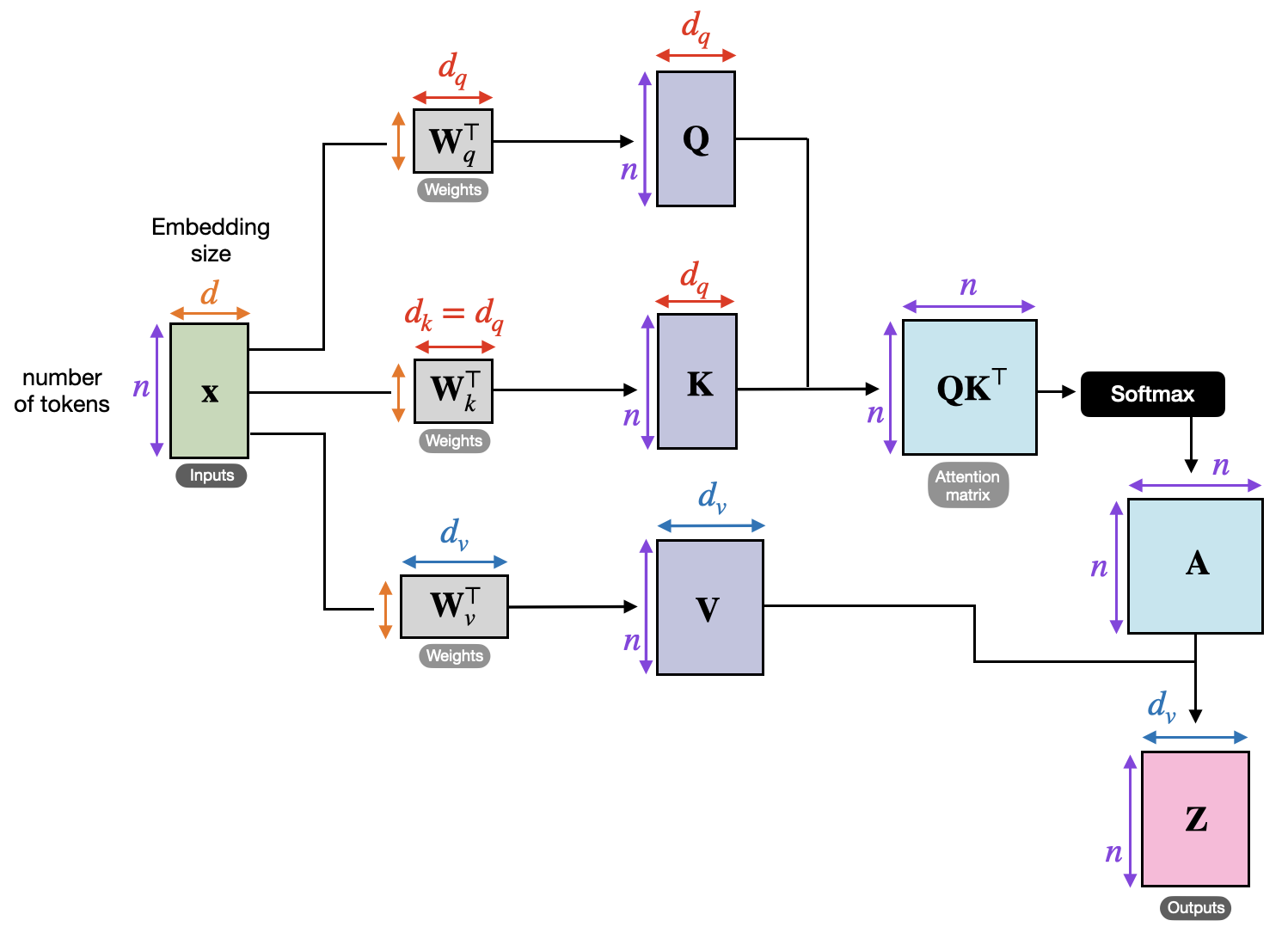
Now, the illustration above corresponds to the self-attention mechanism used in transformers. One particular flavor of this attention mechanism we have yet to discuss is cross-attention.
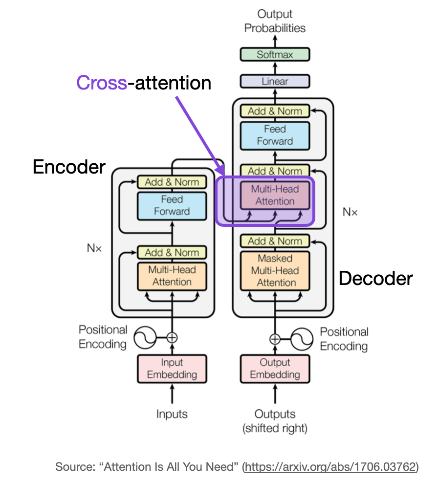
What is cross-attention, and how does it differ from self-attention?
In self-attention, we work with the same input sequence. In cross-attention, we mix or combine two different input sequences. In the case of the original transformer architecture above, that’s the sequence returned by the encoder module on the left and the input sequence being processed by the decoder part on the right.
Note that in cross-attention, the two input sequences \(\mathbf{x}_1\) and \(\mathbf{x}_2\) can have different numbers of elements. However, their embedding dimensions must match.
The figure below illustrates the concept of cross-attention. If we set \(\mathbf{x}_1 = \mathbf{x}_2\), this is equivalent to self-attention.
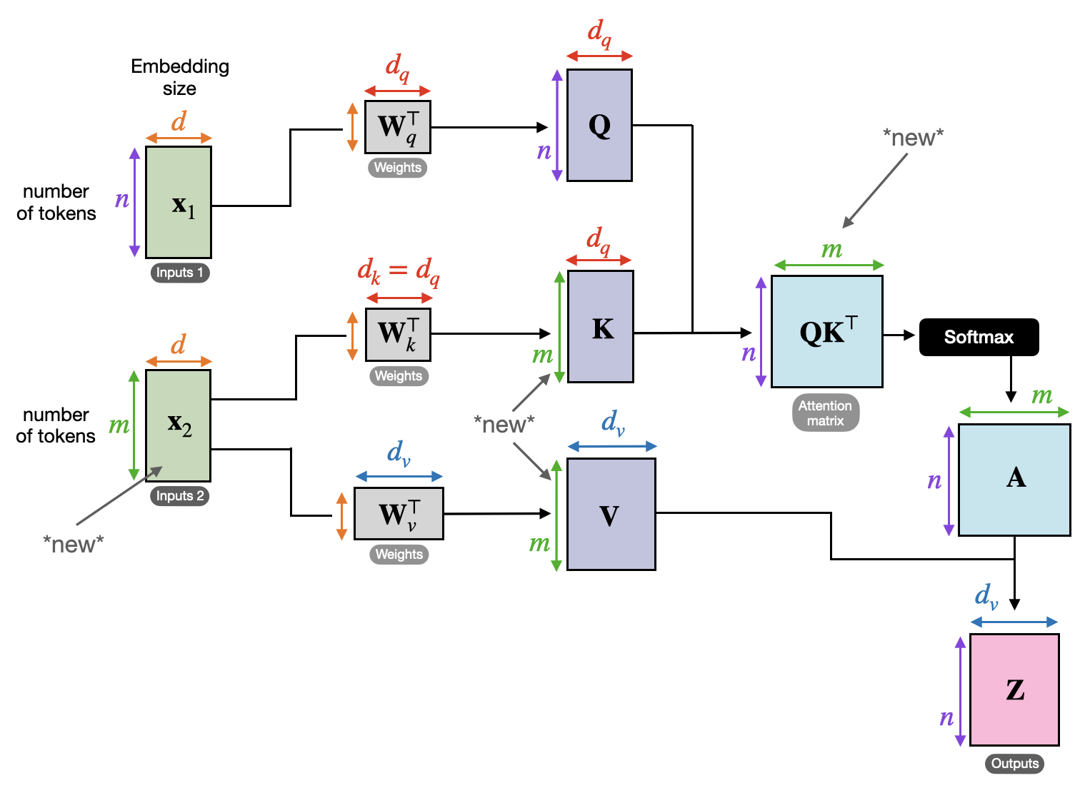
(Note that the queries usually come from the decoder, and the keys and values usually come from the encoder.)
How does that work in code? Previously, when we implemented the self-attention mechanism at the beginning of this article, we used the following code to compute the query of the second input element along with all the keys and values as follows:
In:
torch.manual_seed(123)

d = embedded_sentence.shape[1]
print("embedded_sentence.shape:", embedded_sentence.shape:)

d_q, d_k, d_v = 24, 24, 28

W_query = torch.rand(d_q, d)
W_key = torch.rand(d_k, d)
W_value = torch.rand(d_v, d)

x_2 = embedded_sentence[1]
query_2 = W_query.matmul(x_2)
print("query.shape", query_2.shape)

keys = W_key.matmul(embedded_sentence.T).T
values = W_value.matmul(embedded_sentence.T).T

print("keys.shape:", keys.shape)
print("values.shape:", values.shape)
Out:
embedded_sentence.shape: torch.Size([6, 16])
queries.shape: torch.Size([24])
keys.shape: torch.Size([6, 24])
values.shape: torch.Size([6, 28])
The only part that changes in cross attention is that we now have a second input sequence, for example, a second sentence with 8 instead of 6 input elements. Here, suppose this is a sentence with 8 tokens.
In:
embedded_sentence_2 = torch.rand(8, 16) # 2nd input sequence

keys = W_key.matmul(embedded_sentence_2.T).T
values = W_value.matmul(embedded_sentence_2.T).T

print("keys.shape:", keys.shape)
print("values.shape:", values.shape)
Out:
keys.shape: torch.Size([8, 24])
values.shape: torch.Size([8, 28])
Notice that compared to self-attention, the keys and values now have 8 instead of 6 rows. Everything else stays the same.
We talked a lot about language transformers above. In the original transformer architecture, cross-attention is useful when we go from an input sentence to an output sentence in the context of language translation. The input sentence represents one input sequence, and the translation represent the second input sequence (the two sentences can different numbers of words).
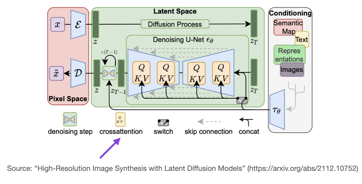
Another popular model where cross-attention is used is Stable Diffusion. Stable Diffusion uses cross-attention between the generated image in the U-Net model and the text prompts used for conditioning as described in High-Resolution Image Synthesis with Latent Diffusion Models – the original paper that describes the Stable Diffusion model that was later adopted by Stability AI to implement the popular Stable Diffusion model.
Conclusion
In this article, we saw how self-attention works using a step-by-step coding approach. We then extended this concept to multi-head attention, the widely used component of large-language transformers. After discussing self-attention and multi-head attention, we introduced yet another concept: cross-attention, which is a flavor of self-attention that we can apply between two different sequences. This is already a lot of information to take in. Let’s leave the training of a neural network using this multi-head attention block to a future article.
Cite / Share
Short Description
In this article, we are going to understand how self-attention works from scratch. This means we will code it ourselves one step at a time. Since its...
BibTeX
@misc{raschka2023understandingandcodingtheselfattenti,
  author = {Raschka, Sebastian},
  title = {Understanding and Coding the Self-Attention Mechanism of Large Language Models From Scratch},
  year = {2023},
  month = {February},
  url = {https://sebastianraschka.com/blog/2023/self-attention-from-scratch.html},
  note = {Accessed: 2026-05-03}
}
Suggested Share Text
Understanding and Coding the Self-Attention Mechanism of Large Language Models From Scratch by Sebastian Raschka: https://sebastianraschka.com/blog/2023/self-attention-from-scratch.html
Read Next
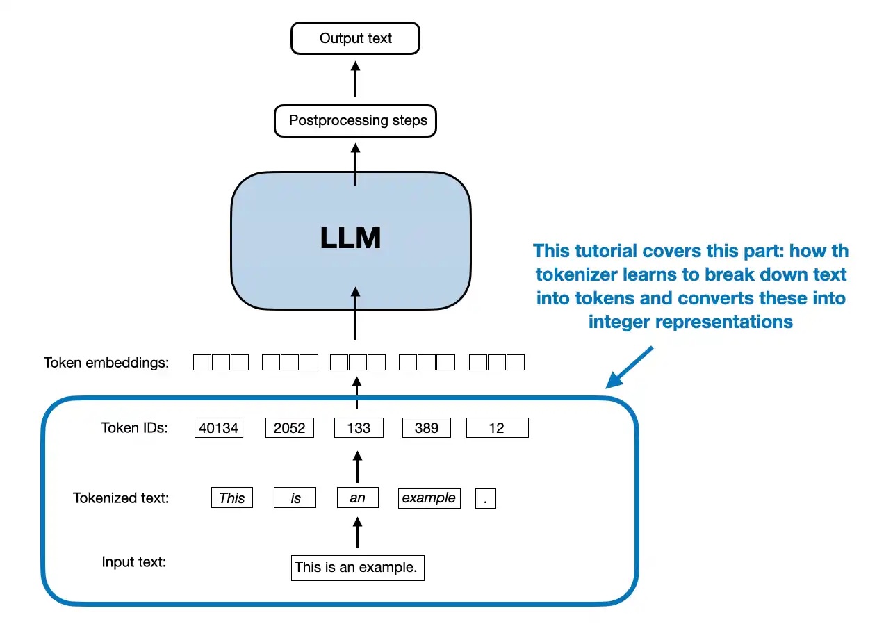 Implementing a BPE Tokenizer From Scratch
Continue with tokenization, the other early building block in an LLM pipeline.
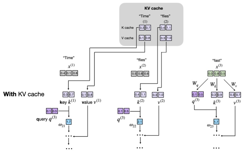 Understanding and Coding the KV Cache in LLMs from Scratch
See how attention keys and values are reused for efficient generation.
 LLM Architecture Gallery
Browse modern architecture diagrams after learning the attention core.

If you read the book and have a few minutes to spare, I'd really appreciate a brief review. It helps us authors a lot!
Your support means a great deal! Thank you!