Optimizing Memory Usage for Training LLMs and Vision Transformers in PyTorch

Peak memory consumption is a common bottleneck when training deep learning models such as vision transformers and LLMs. This article provides a series of techniques that can lower memory consumption by approximately 20x without sacrificing modeling performance and prediction accuracy.

Introduction

In this article, we will be exploring 9 easily-accessible techniques to reduce memory usage in PyTorch. These techniques are cumulative, meaning we can apply them on top of one another.

We will begin working with a vision transformer from PyTorch’s Torchvision library to provide simple code examples that you can execute on your own machine without downloading and installing too many code and dataset dependencies. The self-contained baseline training script consists of ~100 lines of code (ignoring the whitespaces and code comments). All code examples are available here on GitHub.

Here’s an outline of the sections and techniques we are going to cover:

1. Finetuning a Vision Transformer
2. Automatic Mixed-Precision Training
3. Lower-Precision Training
4. Training with Reduced Batch Size
5. Gradient Accumulation and Microbatches
6. Choosing Leaner Optimizers
7. Instantiating Models on the Target Device
8. Distributed Training and Tensor Sharding
9. Parameter Offloading
10. Putting It All Together: Training an LLM

While we are working with a vision transformer here (the ViT-L-16 model from the paper An Image is Worth 16x16 Words: Transformers for Image Recognition at Scale), all the techniques used in this article transfer to other models as well: Convolutional networks, large language models (LLMs), and others.

Furthermore, after introducing one technique at a time using the abovementioned vision transformer example, we will apply these to train a BigBird-Roberta LLM on a text classification task. It wouldn’t be possible to train such a model on consumer hardware without these techniques.

PS: Note that there are many sections in this article. To not bloat this article further, I will keep each section purposefully short but provide links to more detailed articles on the individual topics.

1) Finetuning a Vision Transformer

To simplify the PyTorch code for the experiments, we will be introducing the open-source Fabric library, which allows us to apply various advanced PyTorch techniques (automatic mixed-precision training, multi-GPU training, tensor sharding, etc.) with a handful (instead of dozens) lines of code.

The difference between simple PyTorch code and the modified one to use Fabric is subtle and involves only minor modifications, as highlighted in the code below:

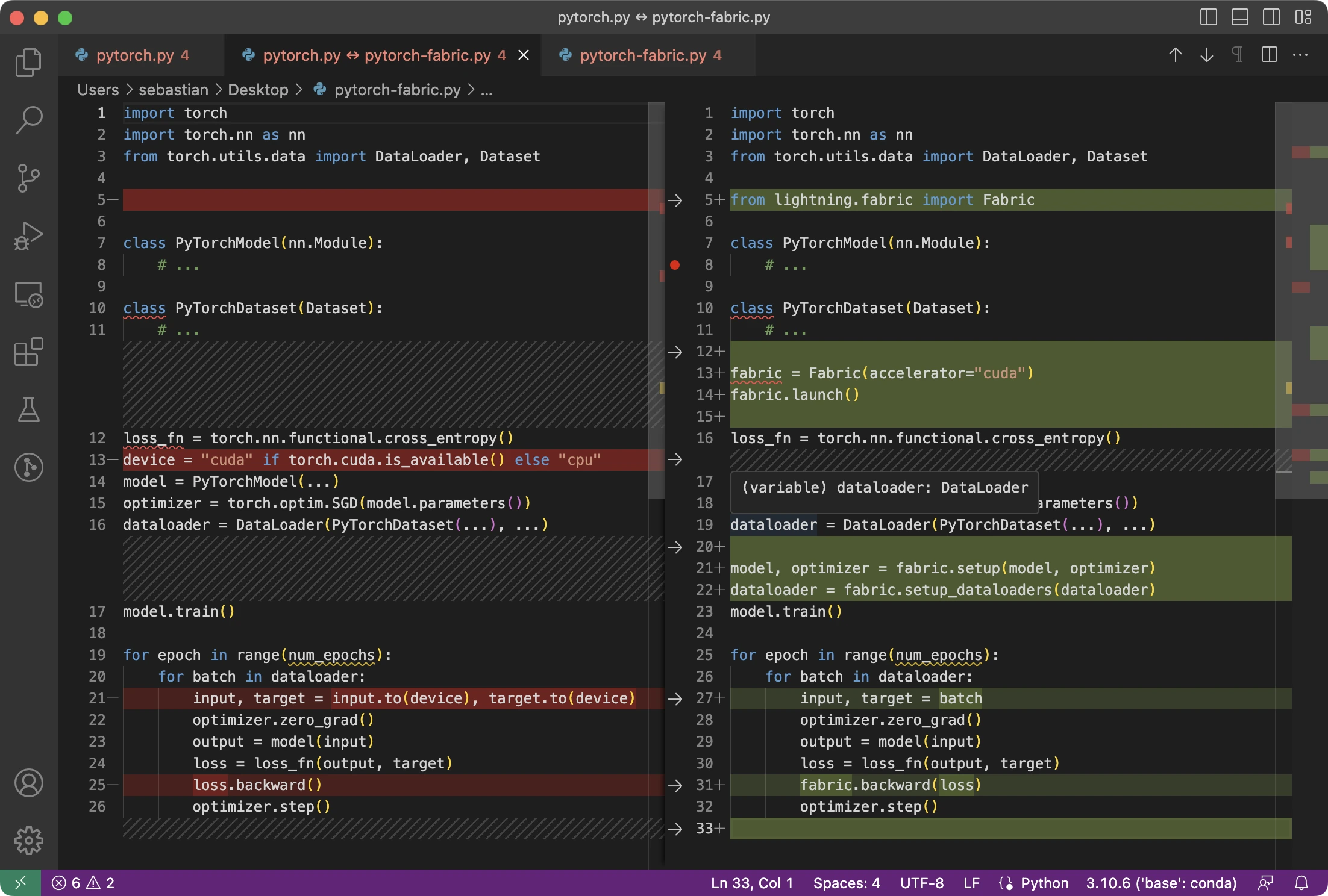
As mentioned above, these minor changes now provide a gateway to utilize advanced features in PyTorch, as we will see in a bit, without restructuring any more of the existing code.

To summarize the figure above, the main 3 steps for converting plain PyTorch code to PyTorch+Fabric are as follows:

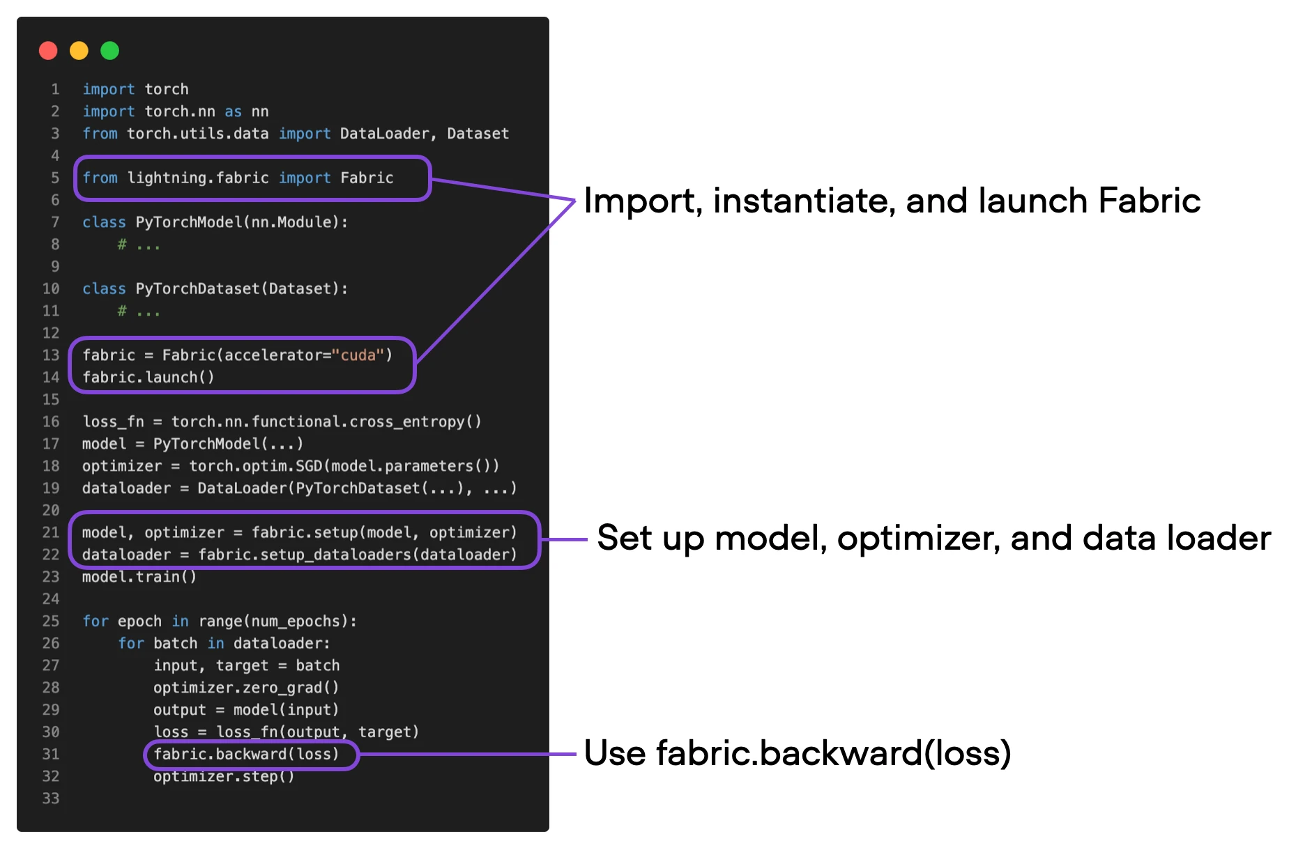
1. Import Fabric and instantiate a Fabric object.
2. Use Fabric to set up the model, the optimizer, and the data loader.
3. Call fabric.backward() on the loss instead of the usual loss.backward()

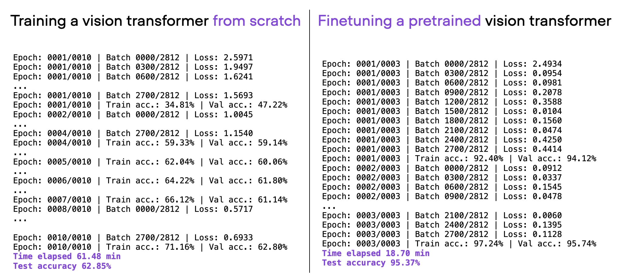
The vision transformer is based on the original ViT architecture, and the code is available here for inspection. Note that we are finetuning the model for classification instead of training it from scratch to optimize predictive performance.

As a quick sanity check, the predictive performance and memory consumption using plain PyTorch and PyTorch with Fabric remains exactly the same (+/- expected fluctuations due to randomness):

Plain PyTorch (01_pytorch-vit.py):

Time elapsed 17.94 min
Memory used: 26.79 GB
Test accuracy 95.85%

PyTorch with Fabric (01-2_pytorch-fabric.py)

Time elapsed 17.88 min
Memory used: 26.84 GB
Test accuracy 96.06%

As an optional exercise, you are welcome to experiment with the code and replace

model = vit_l_16(weights=ViT_L_16_Weights.IMAGENET1K_V1)

with

model = vit_l_16(weights=None)

This will train the same vision transformer architecture from scratch instead of finetuning it. If you carry out this exercise, you’ll see that the prediction accuracy drops from >96% down to ~60%:

2) Automatic Mixed-Precision

In the previous section, we modified our PyTorch code using Fabric. Why go through all this hassle? As we will see below, we can now try advanced techniques, like mixed-precision and distributed training, by only changing one line of code.

We will start with mixed-precision training, which has become the recent norm for training deep neural networks.

Applying Mixed-Precision Training

We can apply mixed-precision training with only one small modification, changing

fabric = Fabric(accelerator="cuda", devices=1)

to the following:

fabric = Fabric(accelerator="cuda", devices=1, precision="16-mixed")

As a result, our memory consumption is reduced from 26.84 GB to 18.21 GB without sacrificing prediction accuracy, as shown below.

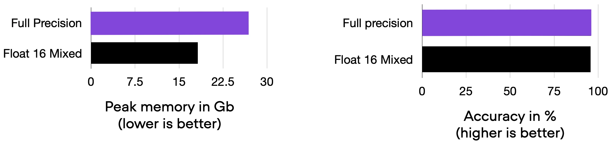
Title: Comparing 01-2_pytorch-fabric.py and 02_mixed-precision.py

As a bonus, mixed-precision training doesn’t only reduce memory usage but also reduces the runtime 6-fold (from 17.88 min to 3.45 min), which is a nice, added benefit; however, the focus of this particular article is on memory consumption to not complicate it further.

What Is Mixed-Precision Training?

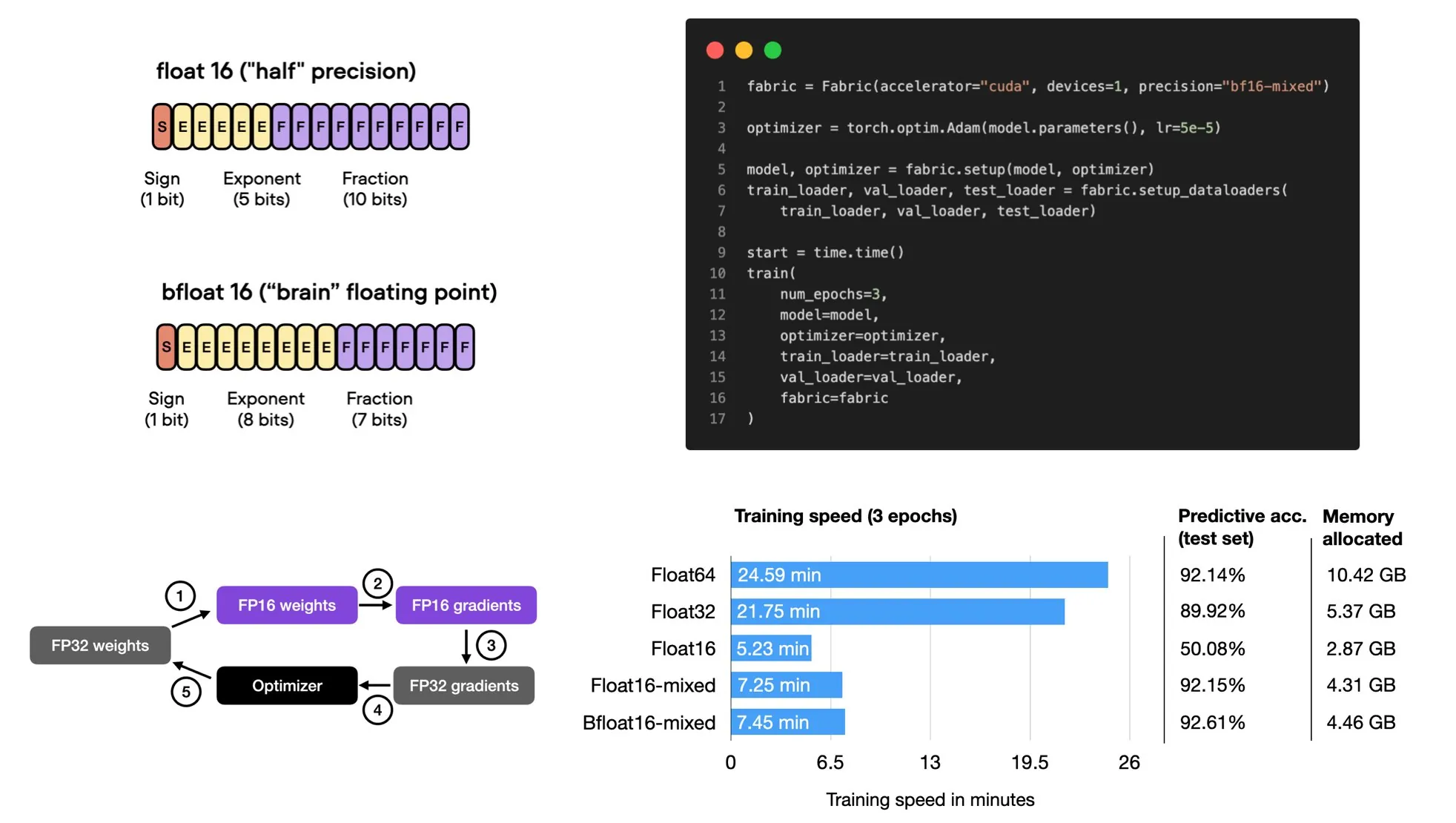
Mixed precision training uses both 16-bit and 32-bit precision to ensure no loss in accuracy. The computation of gradients in the 16-bit representation is much faster than in the 32-bit format and saves a significant amount of memory. This strategy is beneficial, especially when we are memory or compute-constrained.

It’s called “mixed-“rather than “low-“precision training because we don’t transfer all parameters and operations to 16-bit floats. Instead, we switch between 32-bit and 16-bit operations during training, hence, the term “mixed” precision.

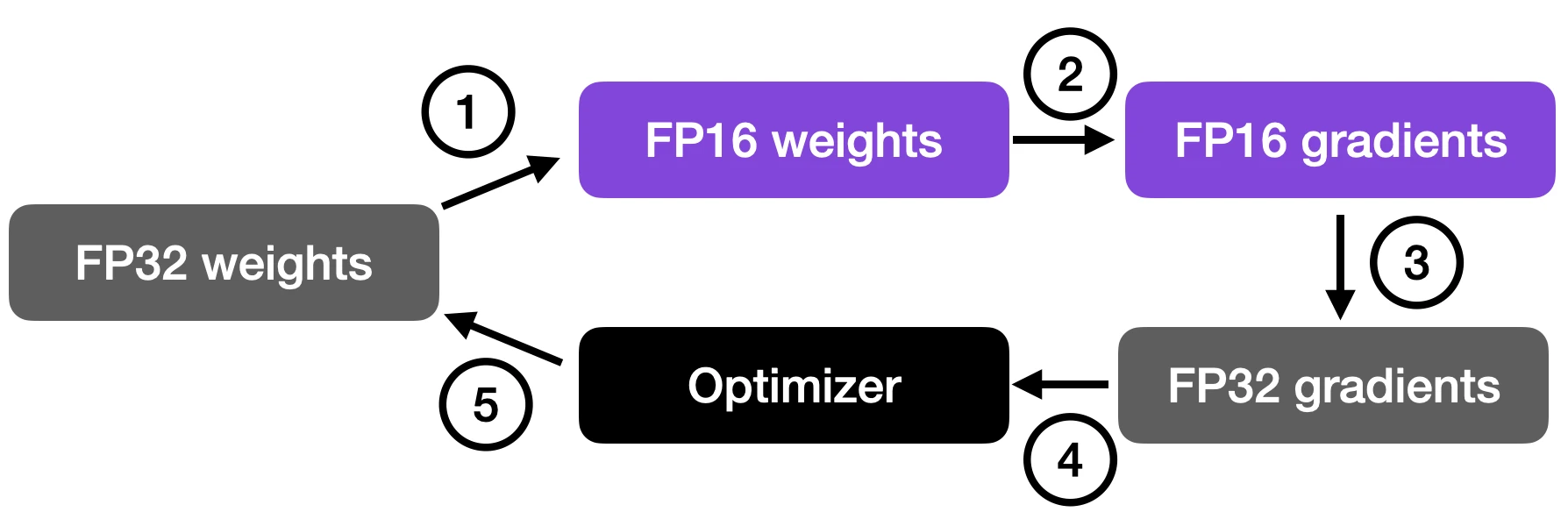
As illustrated in the figure below, mixed-precision training involves converting weights to lower-precision (FP16) for faster computation, calculating gradients, converting gradients back to higher-precision (FP32) for numerical stability, and updating the original weights with the scaled gradients.

This approach allows for efficient training while maintaining the accuracy and stability of the neural network.

For additional details, I recommend reading my more detailed standalone article Accelerating Large Language Models with Mixed-Precision Techniques, where I dive deeper into the underlying concepts.

3) Lower-Precision Training

We can also take it a step further and try running with “full” lower 16-bit precision (instead of mixed-precision, which converts intermediate results to a 32-bit representation.)

We can enable lower-precision training by changing

fabric = Fabric(accelerator="cuda", precision="16-mixed")

to the following:

fabric = Fabric(accelerator="cuda", precision="16-true")

However, you may notice that when running this code, you’ll encounter NaN values in the loss:

Epoch: 0001/0001 | Batch 0000/0703 | Loss: 2.4105
Epoch: 0001/0001 | Batch 0300/0703 | Loss: nan
Epoch: 0001/0001 | Batch 0600/0703 | Loss: nan
...

This is because regular 16-bit floats can only represent numbers between -65,504 and 65,504:

In [1]: import torch

In [2]: torch.finfo(torch.float16)
Out[2]: finfo(resolution=0.001, min=-65504, max=65504, eps=0.000976562, smallest_normal=6.10352e-05, tiny=6.10352e-05, dtype=float16)

So, to avoid the NaN issue, we can use the “bf16-true” setting.

fabric = Fabric(accelerator="cuda", precision="bf16-true")

As a result, we can reduce the memory consumption even further down to 13.82 GB (again, without sacrificing accuracy):

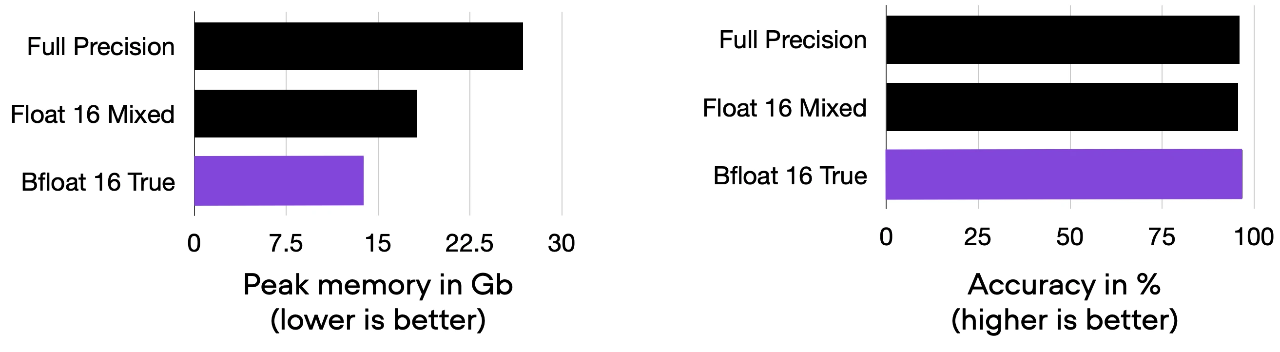
Title: Comparing 03_bfloat16.py to the previous codes

What Is Bfloat16?

The “bf16” in "bf16-mixed" stands for Brain Floating Point (bfloat16). Google developed this format for machine learning and deep learning applications, particularly in their Tensor Processing Units (TPUs). Bfloat16 extends the dynamic range compared to the conventional float16 format at the expense of decreased precision.

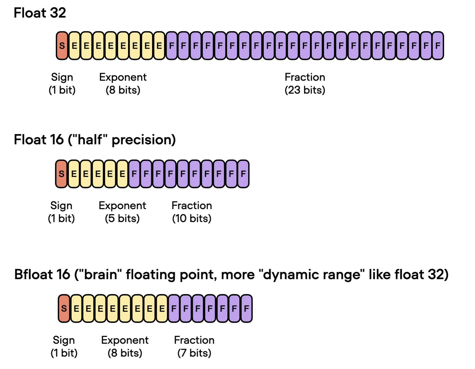
The extended dynamic range helps bfloat16 to represent very large and very small numbers, making it more suitable for deep learning applications where a wide range of values might be encountered. However, the lower precision may affect the accuracy of certain calculations or lead to rounding errors in some cases. But in most deep learning applications, this reduced precision has minimal impact on modeling performance.

While bfloat16 was originally developed for TPUs, this format is now supported by several NVIDIA GPUs as well, beginning with the A100 Tensor Core GPUs, which are part of the NVIDIA Ampere architecture.

You can check whether your GPU supports bfloat16 via the following code:

>>> import torch
>>> torch.cuda.is_bf16_supported()
True

4) Reducing the Batchsize

Let’s tackle one of the big elephants in the room: why don’t we simply reduce the batch size? This is usually always an option to reduce memory consumption. However, it can sometimes result in worse predictive performance since it alters the training dynamics. (For more details, see Lecture 9.5 in my Deep Learning Fundamentals course.)

Either way, let’s reduce the batch size to see how that affects the results. It turns out we can lower the batch size to 16, which brings memory consumption down to 5.69 GB, without sacrificing performance:

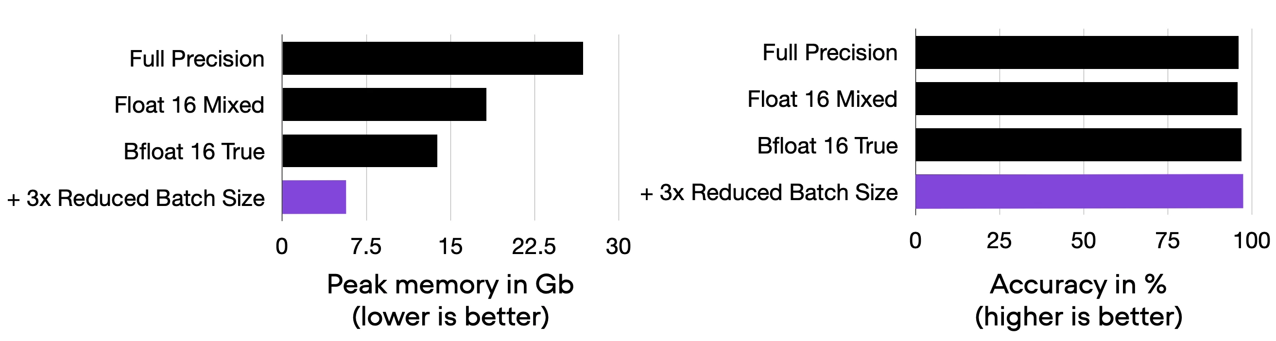
Title: Comparing 04_lower-batchsize.py to the previous codes.

5) Using Gradient Accumulation to Create Microbatches

Gradient accumulation is a way to virtually increase the batch size during training, which is very useful when the available GPU memory is insufficient to accommodate the desired batch size. Note that this only affects the runtime, not the modeling performance.

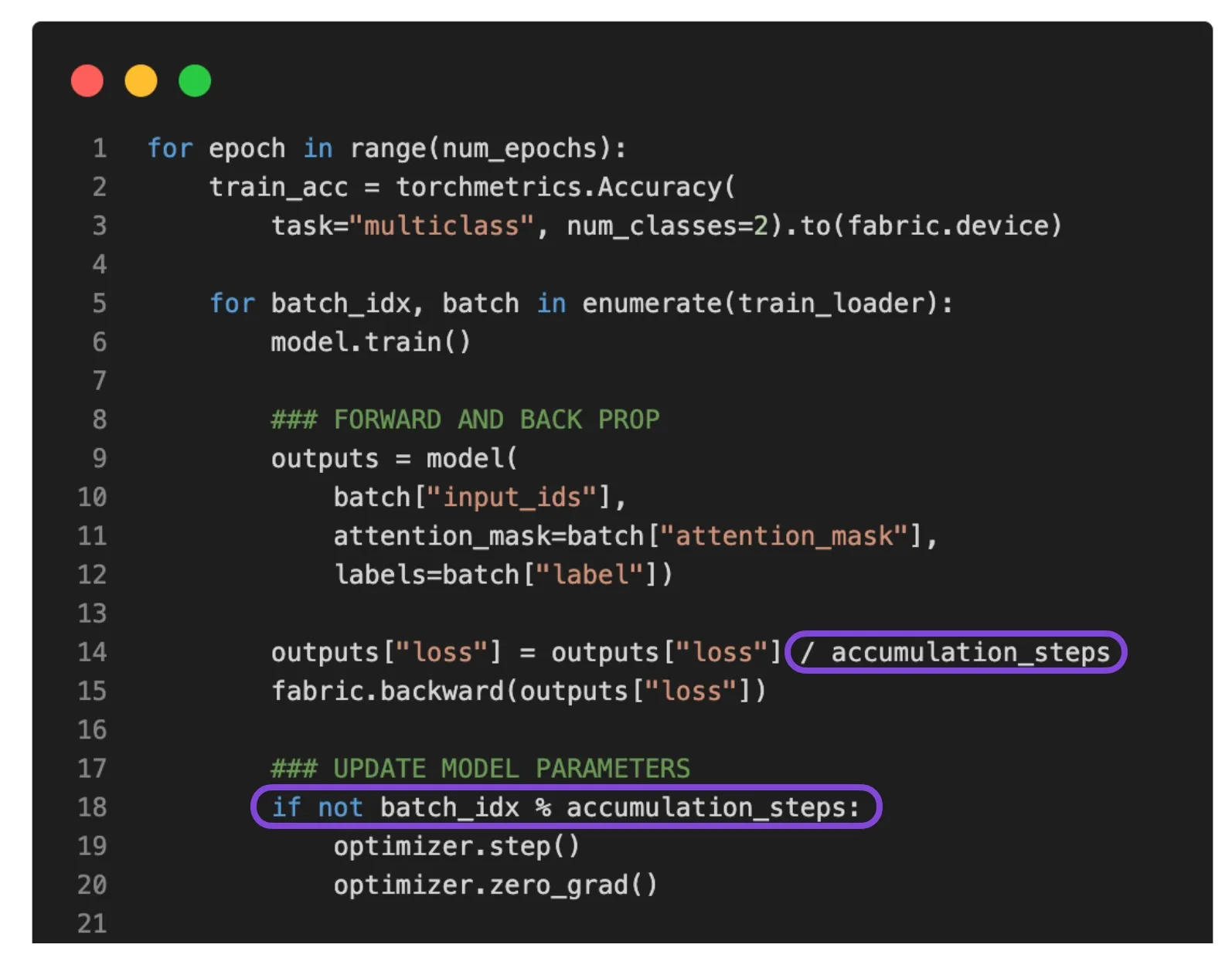
In gradient accumulation, gradients are computed for smaller batches and accumulated (usually summed or averaged) over multiple iterations instead of updating the model weights after every batch. Once the accumulated gradients reach the target “virtual” batch size, the model weights are updated with the accumulated gradients.

To enable gradient accumulation, there are only two small modifications to the forward and backward pass required:

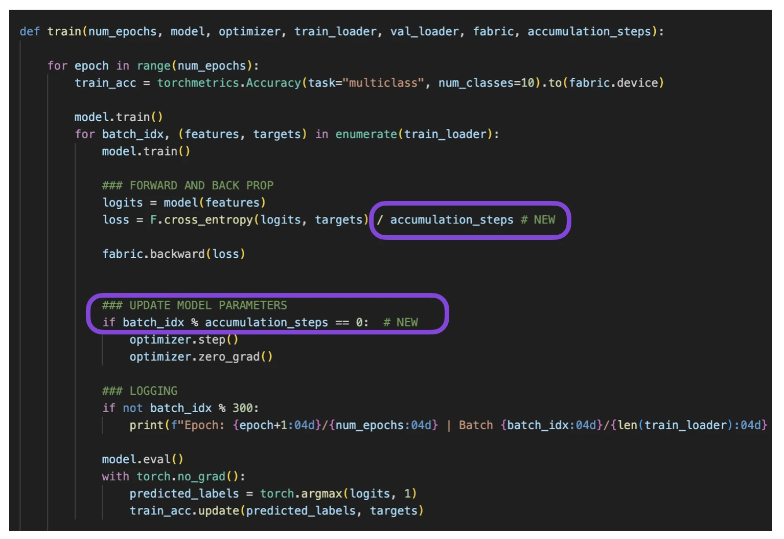
Title: Code modification in 05_gradient-accum.py

I covered gradient accumulation in more detail in my article Finetuning LLMs on a Single GPU Using Gradient Accumulation.

Using an effective batch size of 16 and 4 accumulation steps means we will use an actual batch size of 4 (since 16 / 4 = 4).

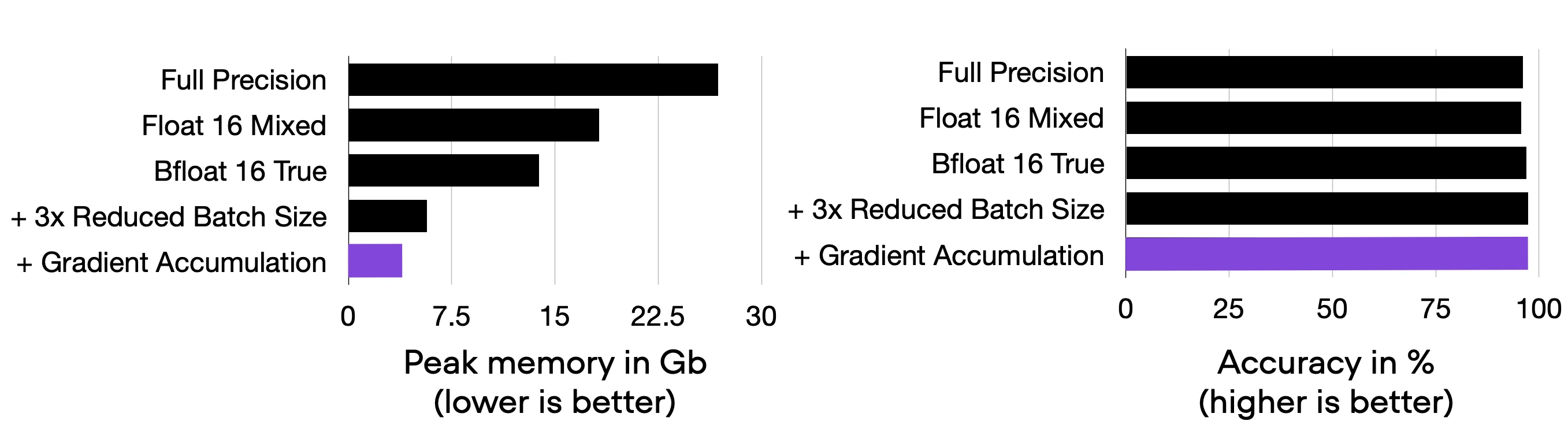
Title: Result of 05_gradient-accum.py

A disadvantage of this technique is that it increases the runtime from 3.96 min to 12.91 min.

Of course, we could even go smaller and e 16 accumulation steps. This would lead to a microbatch size of 1, reducing the memory size further (about 75%), but I’ll leave this as an optional exercise.

6) Using a Leaner Optimizer

Did you know that the popular Adam optimizer comes with additional parameters? For instance, Adam has 2 additional optimizer parameters (a mean and a variance) for each model parameter.

So, by swapping Adam with a stateless optimizer like SGD, we can reduce the number of parameters by 2/3, which can be quite significant when working with vision transformers and LLMs.

The downside of plain SGD is that it usually has worse convergence properties. So, let’s swap Adam with SGD and introduce a cosine decay learning rate scheduler to compensate for this and achieve better convergence.

In short, we will be swapping the previously used Adam optimizer:

optimizer = torch.optim.Adam(model.parameters(), lr=5e-5)

with an SGD optimizer plus scheduler:

optimizer = torch.optim.SGD(model.parameters(), lr=0.01)

num_steps = NUM_EPOCHS * len(train_loader)
scheduler = torch.optim.lr_scheduler.CosineAnnealingLR(
    optimizer, T_max=num_steps)

With this change, we are able to have the peak memory consumption while maintaining ~97% classification accuracy:

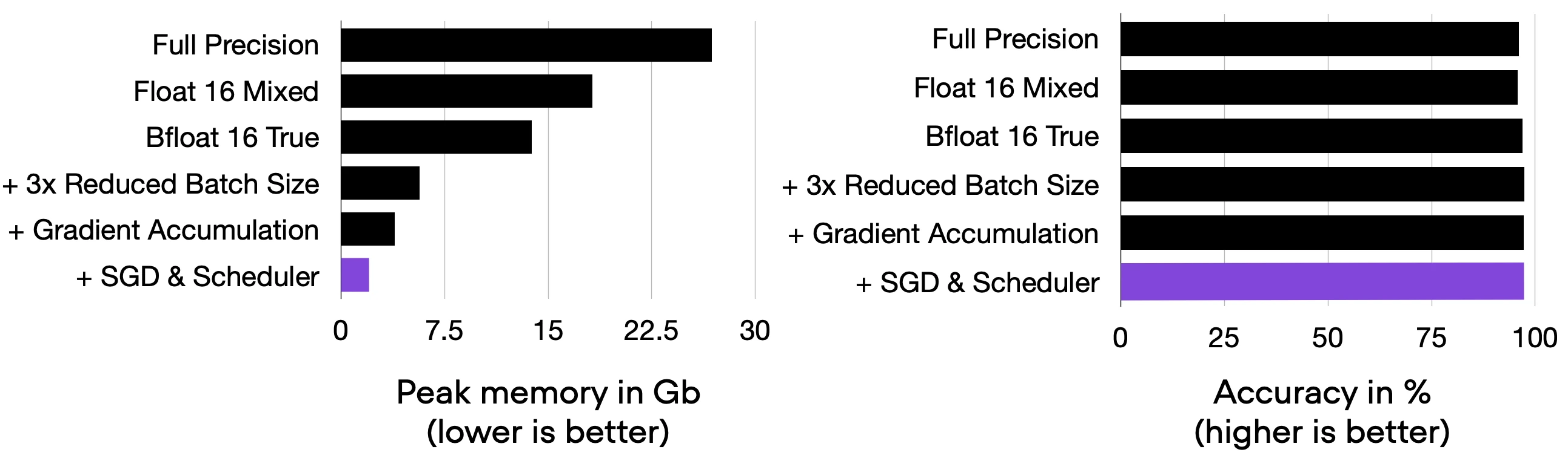
Title: Result of 06_sgd-with-scheduler.py

If you want to learn more, I discussed learning rate schedulers (including cosine decay with a 1-cycle schedule) in more detail in my Unit 6.5 of my Deep Learning Fundamentals class.

7) Creating the Model on the Target Device with Desired Precision

When we instantiate a model in PyTorch, we usually create it on the CPU device first, and then we transfer it onto the target device and convert it to the desired precision:

model = vit_l_16(weights=ViT_L_16_Weights.IMAGENET1K_V1)
model.cuda().float16()

This can be inefficient considering the intermediate model representation in full precision on the CPU. Instead, we can directly create the model in desired precision on the target device (e.g., GPU) using the init_module context in Fabric:

import lightning as L

fabric = Fabric(accelerator="cuda", devices=1, precision="16-true")

with fabric.init_module():
    model = vit_l_16(weights=ViT_L_16_Weights.IMAGENET1K_V1)

In this specific case (model), the peak memory during the forward pass is larger than the model size in its full precision representation. So, we will benchmark the fabric.init_module approach just for the model loading itself.

• GPU Peak memory without init_module: 1.24 GB (07_01_init-module.py)

• GPU Peak memory with init_module: 0.65 GB (07_03_init-module.py)

As we can see based on the results above, in this case, init_module reduces the peak memory requirements for model loading by 50%. We will be making use of this technique later in this article.

For more details about init_module, please see the more detailed article on Efficient Initialization of Large Models.

8) Distributed Training and Tensor Sharding

The next modification we are going to try is multi-GPU training. It becomes beneficial if we have multiple GPUs at our disposal since it allows us to train our models even faster.

However, here, we are mainly interested in the memory saving. So, we are going to use a more advanced, distributed multi-GPU strategy called Fully Sharded Data Parallelism (FSDP), which utilizes both data parallelism and tensor parallelism for sharding large weight matrices across multiple devices.

Note that the model is already very small, which is why we wouldn’t see any major effect when adding this technique to the code from section 7 above. Hence, to focus on the pure effect of sharding, we are going to compare this code to the full precision baseline from section 1.

We are changing

fabric = Fabric(accelerator="cuda", devices=1)

to

auto_wrap_policy = partial(
    transformer_auto_wrap_policy,
    transformer_layer_cls={EncoderBlock})
    
strategy = FSDPStrategy(
    auto_wrap_policy=auto_wrap_policy,      
    activation_checkpointing=EncoderBlock)

fabric = Fabric(accelerator="cuda", devices=4, strategy=strategy)

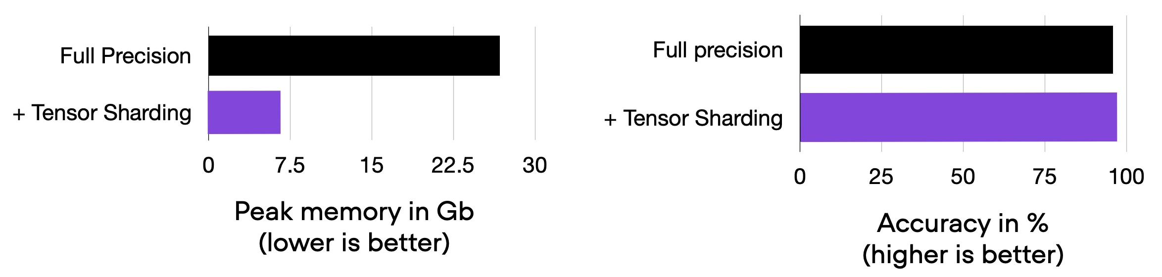
Title: Result of 08_fsdp-with-01-2.py

Note that instead of manually defining the strategy above, we can also just use the following, which automatically determines which layers to shard:

fabric = Fabric(accelerator="cuda", devices=4, strategy="fsdp")

Understanding Data Parallelism and Tensor Parallelism

In data parallelism, the mini-batch is divided, and a copy of the model is available on each of the GPUs. This process speeds up model training as multiple GPUs work in parallel.

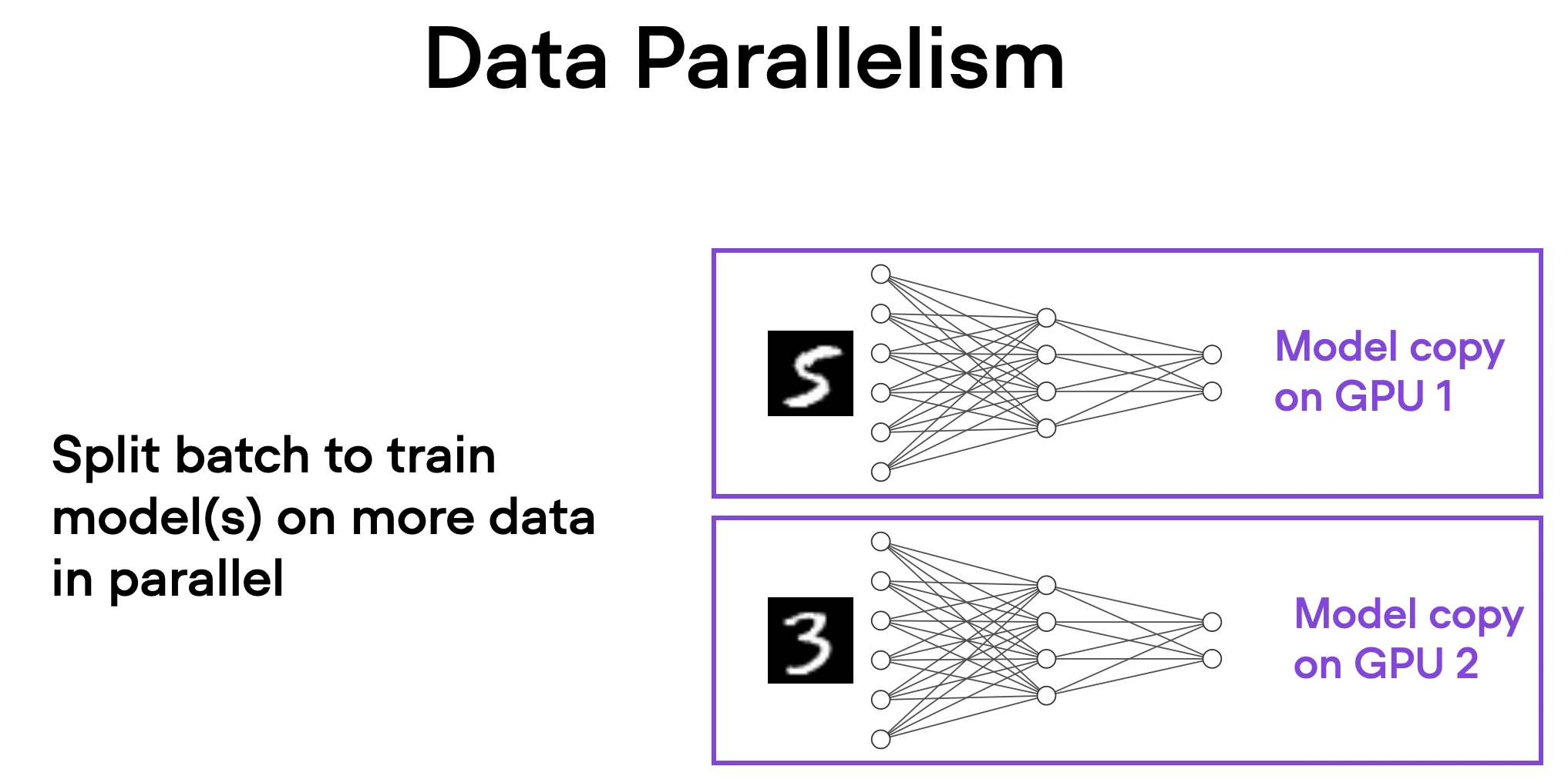
Here’s how it works in a nutshell:

1. The same model is replicated across all the GPUs.
2. Each GPU is then fed a different subset of the input data (a different mini-batch).
3. All GPUs independently perform forward and backward passes of the model, computing their own local gradients.
4. Then, the gradients are collected and averaged across all GPUs.
5. The averaged gradients are then used to update the model’s parameters.

The primary advantage of this approach is speed. Since each GPU is processing a unique mini-batch of data concurrently with the others, the model can be trained on more data in less time. This can significantly reduce the time required to train our model, especially when working with large datasets.

However, data parallelism has some limitations. Most importantly, each GPU must have a complete copy of the model and its parameters. This places a limit on the size of the model we can train, as the model must fit within a single GPU’s memory – this is not feasible for modern ViTs or LLMs.

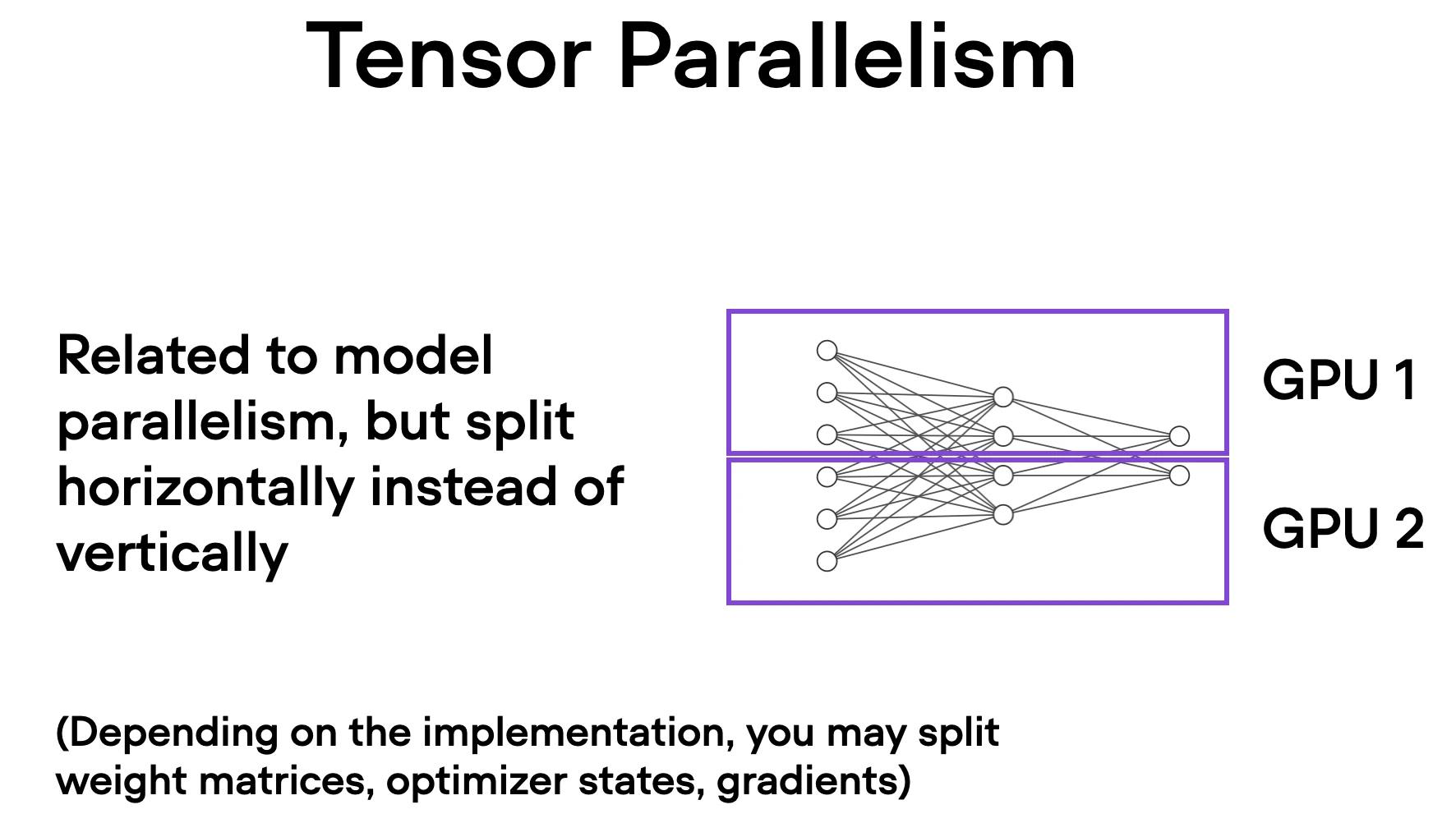
Unlike data parallelism, which involves splitting a mini-batch across multiple devices, tensor parallelism divides the model itself across GPUs. In data parallelism, every GPU needs to fit the entire model, which can be a limitation when training larger models. Tensor parallelism, on the other hand, allows for training models that might be too large for a single GPU by breaking up the model and distributing it across multiple devices.

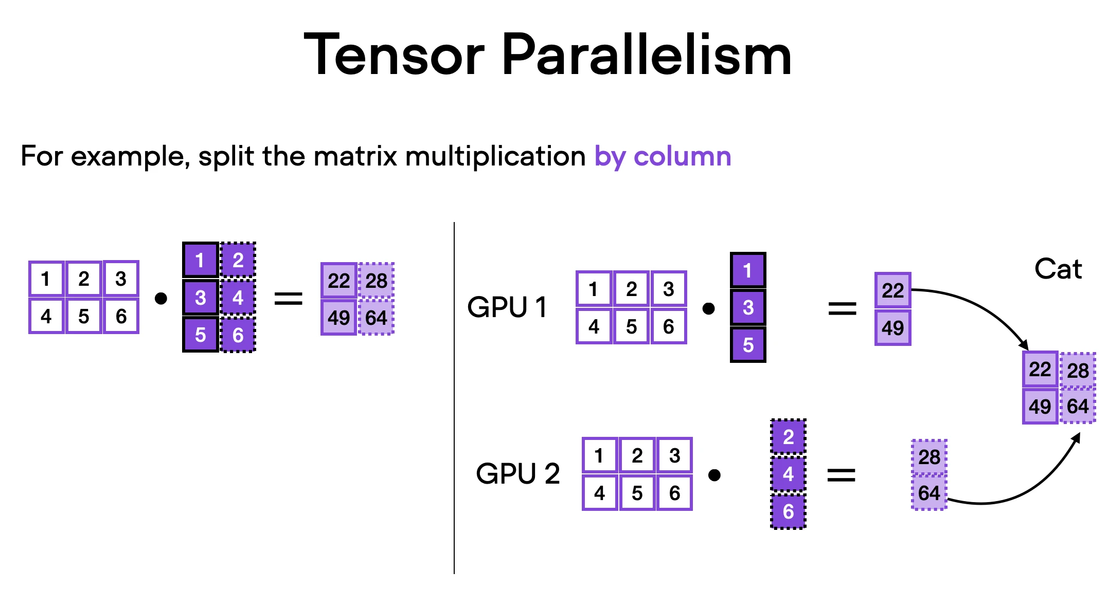
How does it work? Think of matrix multiplication. There are two ways to distribute it – by row or by column. For simplicity, let’s consider distribution by column. For instance, we can break down a large matrix multiplication operation into separate computations, each of which can be carried out on a different GPU, as shown in the figure below. The results are then concatenated to get the original result, effectively distributing the computational load.

9) Parameter Offloading

In addition to the FSDP strategy explained in the previous section above, we can also offload optimizer parameters to the CPU, which we can enable by changing

strategy = FSDPStrategy(
    auto_wrap_policy=auto_wrap_policy,      
    activation_checkpointing=EncoderBlock,
)

to

strategy = FSDPStrategy(
    auto_wrap_policy=auto_wrap_policy,      
    activation_checkpointing=EncoderBlock,
    cpu_offload=True
)

This reduces the memory consumtion from 6.59 GB to 6.03 GB:

Title: Result of 09_fsdp-cpu-offload-with-01-2.py.

The only slight downside is that it increases the runtime from 5.5 min to 8.3 min.

10) Putting it All Together & Training an LLM

In the previous sections, we covered a lot of ground by optimizing a vision transformer. Of course, some of you may also want to know whether these techniques apply to LLMs. Of course, they do!

We use many of these tricks in our Lit-LLaMA and Lit-GPT repositories, which support LLaMA, Falcon, Pythia, and other popular models. Still, to create a more general example, we will be finetuning an LLM from the popular HF transformers library for classifying the sentiment of IMDb movie reviews.

For example, if you use the above-mentioned techniques, you can train a DistilBERT classifier using only 1.15 Gb memory (bonus_distilbert-after.py) instead of 3.99 Gb (bonus_bigbird-before.py).

Or, more impressively, by applying the techniques to a BigBird model from the transformers library, BigBird consumes only 4.03 GB (bonus_bigbird-after.py)!

  strategy = FSDPStrategy(
        cpu_offload=True
   )

   fabric = Fabric(
        accelerator="cuda",
        devices=4,
        strategy=strategy,
         precision="bf16-true"
   )

   with fabric.init_module():
       model = AutoModelForSequenceClassification.from_pretrained(
            "google/bigbird-roberta-base", num_labels=2)

(I would have included the performance without these techniques as a reference, but it’s not possible to run this model without the abovementioned optimizations.)

Conclusion

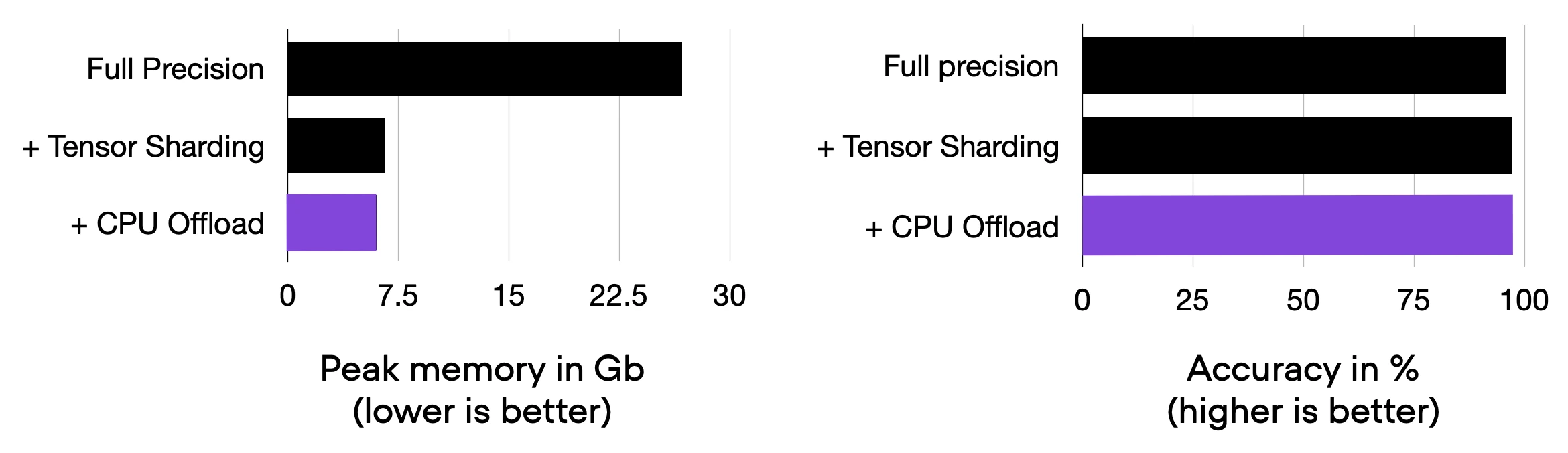
This article showcased 9 techniques to reduce the memory consumption of PyTorch models. When applying these techniques to a vision transformer, we reduced the memory consumption 20x on a single GPU. And we saw that tensor sharding across GPUs could even lower memory consumption. The same optimizations also enabled training a BigBird LLM using only 4 GB of peak GPU RAM.

None of these techniques are model-specific and can be used with practically any PyTorch training script. And using the open-source Fabric library, most of these optimizations can be enabled with a single line of code.