Comparing Different Automatic Image Augmentation Methods in PyTorch
One of the best ways to reduce overfitting is to collect more (good-quality) data. However, collecting more data is not always feasible or can be very expensive. A related technique is data augmentation.
Data augmentation involves generating new data records or features from existing data, expanding the dataset without collecting more data. It helps improve model generalization by creating variations of original input data and making it harder to memorize irrelevant information from training examples or features. Data augmentation is common for image and text data, but also exists for tabular data.
Data augmentation is a key tool in reducing overfitting, whether it’s for images or text. This article compares four automatic image augmentation techniques in PyTorch: AutoAugment, RandAugment, AugMix, and TrivialAugment.
(Why AutoAugment, RandAugment, AugMix, and TrivialAugment? I recently shared my good experiences with AutoAugment. As a follow-up, suggestions led me down the rabbit hole of checking out the other related methods provided in the PyTorch/torchvision library.)
Comparing AutoAugment, RandAugment, AugMix, and TrivialAugment
As mentioned above, this article compares four related data augmentation techniques for image data. All four methods are implemented in the core PyTorch/torchvision library, so they are easy to adopt.
Before we discuss how these methods work in detail, let’s cut to the chase and look at the performance of these methods side by side. I used a very simple ResNet-18 without bells and whistles for this performance comparison. Furthermore, I omitted other techniques to reduce overfitting to keep things simple. (If you are curious about different methods to reduce overfitting, I discuss more than a dozen approaches in my new book Machine Learning Q and AI.)
Code
The code for running the experiment is quite simple, and you can find it here on GitHub if you want to run, adapt, or modify these experiments.
To avoid clutter, I am only showing and summarizing the main parts. You can find the fully self-contained, executable code here on GitHub:
import torch, torchvision
from torchvision import transforms
import lightning as L

## Dataset
train_transform = torchvision.transforms.Compose(
    [
        transforms.Resize(32),
        # One of the following:
        #   1) Nothing
        #   2) transforms.AutoAugment()
        #   3) transforms.RandAugment()
        #   4) transforms.AugMix()
        #   5) transforms.TrivialAugmentWide()
        transforms.ToTensor(),

    ]
)

valid_and_test_transform = transforms.Compose(
    [
        transforms.Resize(32),
        transforms.ToTensor(),
    ]
)

L.seed_everything(123)
dm = Cifar10DataModule(
    batch_size=256,
    train_transform=train_transform,
    valid_and_test_transform=valid_and_test_transform,
    num_workers=4
)

## Model
pytorch_model = torchvision.models.resnet18(weights=None)
pytorch_model.fc = torch.nn.Linear(512, 10)
lightning_model = LightningModel(model=pytorch_model, learning_rate=0.05)

## Training
trainer = L.Trainer(
    max_epochs=1000,
    accelerator="gpu",
    devices=[0],
    logger=CSVLogger(save_dir="logs/"),
    deterministic=True,
)
trainer.fit(model=lightning_model, datamodule=dm)

## Model evaluation
trainer.test(model=lightning_model, datamodule=dm)
As you can see above, I used the same hyperparameters (batch size and learning rate) for all four training scenarios. In addition, I replaced the last layer of the ResNet-18 model provided by PyTorch/torchvision with a layer with 10 output nodes (since CIFAR-10 only has 10 classes).
To keep this blog article concise and focused, I will not explain the code in detail. However, as you know, I am more than happy to chat more about the code if there are any questions. Please feel free to reach out via the accompanying GitHub Discussion forum if you have any questions or comments.
Results
A picture is worth a thousand words, so let’s examine the results below.
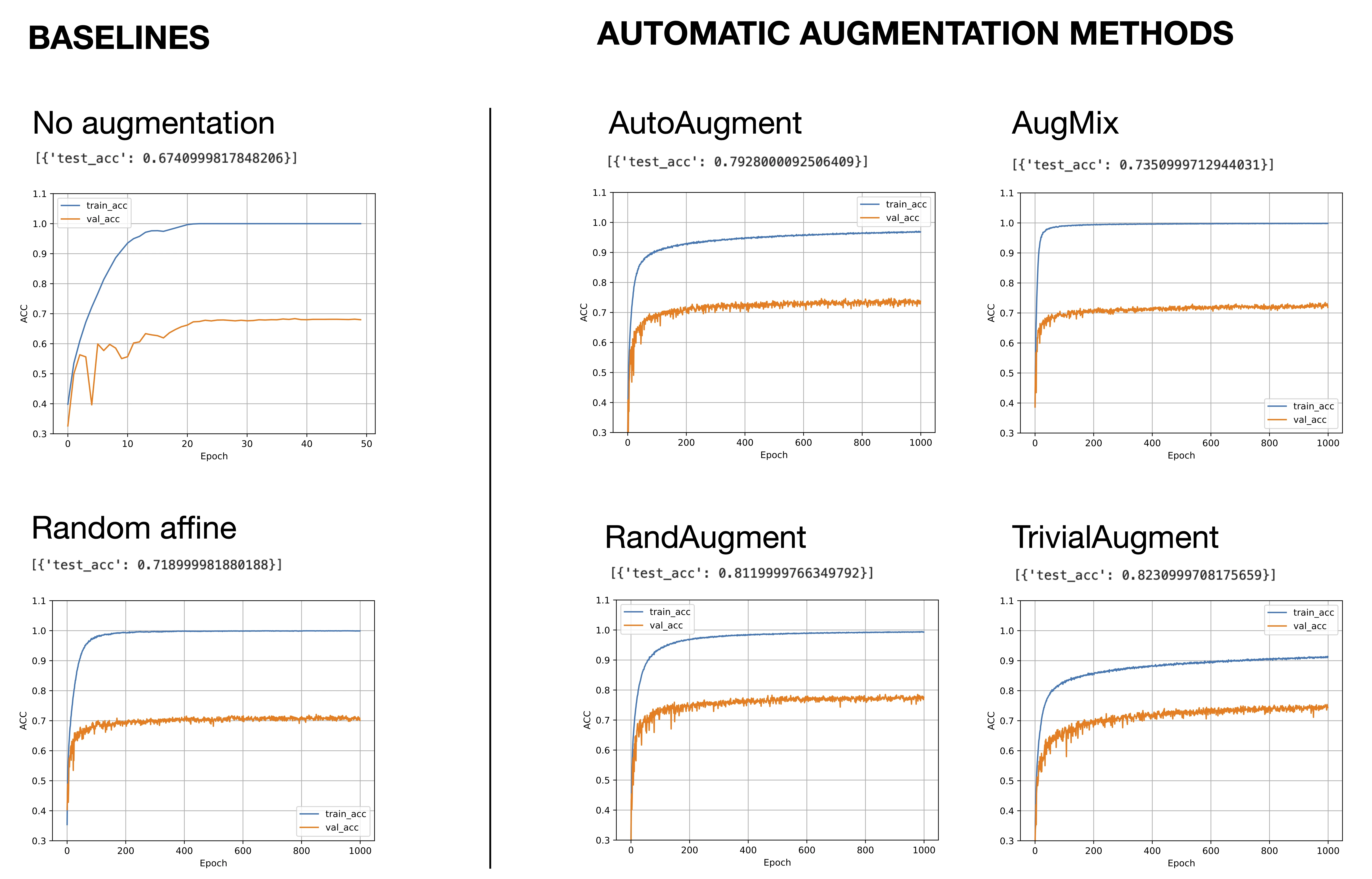
It appears that Autoaugment improves the test set accuracy about 12% compared to no augmentation, which is a huge improvement. RandAugment, which is the successor of AutoAugment improves the performance by another 2 percentage points. And TrivialAugment, a newer and much simpler alternative performs yet another percent better than RandAugment.
AugMix performs better than no augmentation, but it is not as good as AutoAugment, RandAugment, or TrivialAugment. This is expected since AugMix was developed with distributions shifts (rather than improving the validation accuracy) in mind.
As shown in the figure above, I also included RandomAffine as a baseline. RandomAffine applies a random affine transformation of the image involving random translation, scaling, and shearing. It performs better than no augmentation, but it doesn’t come close to the other augmentation methods (AutoAugment, RandAugment, and TrivialAugment).
Note that I also ran AutoAugment, RandAugment, AugMix, and TrivialAugment for 2000 epochs since the positive slope of the validation accuracy graphs suggested that more extended training could improve the predictive performance further (results not shown). However, the test set performance after 2000 epochs did not improve compared to the 1000-epoch experiments above.
Limitations
The apparent grain of salt here is that I only ran these experiments on a single neural network architecture (ResNet-18) and a single dataset (CIFAR-10). Your mileage may vary depending on your model architecture, dataset, and use of other techniques to reduce overfitting.
References
Here are the references and links for the three different data augmentation approaches. The following section will discuss and summarize them in more detail.
AutoAugment
- Paper: Cubuk, Zoph, Mane, Vasudevan, Le (Apr 2019) AutoAugment: Learning Augmentation Policies from Data, https://arxiv.org/abs/1805.09501.
- Implementation: torchvision.transforms.AutoAugment
RandAugment
- Paper: Cubuk, Zoph, Shlens, Le (Nov 2019). RandAugment: Practical Automated Data Augmentation With A Reduced Search Space, https://arxiv.org/abs/1909.13719
- Implementation: torchvision.transforms.RandAugment
AugMix
- Paper: Hendrycks, Mu, Cubuk, Zoph, Gilmer, Lakshminarayanan (2020). AugMix: A Simple Data Processing Method to Improve Robustness and Uncertainty, https://arxiv.org/abs/1912.02781
- Impleentation: torchvision.transforms.AugMix
TrivialAugment
- Paper: Mueller, Hutter (Aug 2021). TrivialAugment: Tuning-free Yet State-of-the-Art Data Augmentation, https://arxiv.org/abs/2103.10158.
- Implementation: torchvision.transforms.TrivialAugmentWide
Method Summaries and Comparisons
This section briefly outlines how the different automatic or learned image augmentations work and compare to each other based on the literature referenced above.
AutoAugment
In this paper, the authors learn combinations of image transformations that optimize the validation set accuracy on a given dataset. The candidates for the transformation cocktails are shearing, translation, rotation, contrast, pixel inversion, histogram equalization, solarization, posterization, color, brightness, sharpness, Cutout, and Sample Pairing.
The search for effective image transformation techniques is a discrete optimization problem that can be approached with techniques such as grid search, random search, reinforcement learning (RL), or evolutionary algorithms.
In AutoAugment, the researchers chose RL and a recurrent neural network as the controller algorithm. The controller was trained to improve validation set accuracy, but since accuracy is not differentiable, policy gradient methods were used to update the RNN.
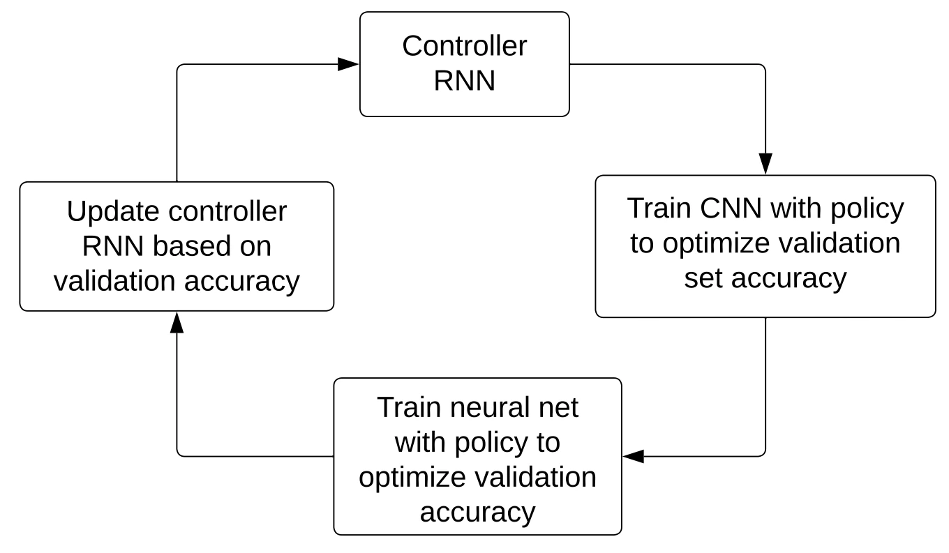
The controller was a 1-layer LSTM with 100 hidden units (details in here). The training utilized PPO (proximal policy optimization).
And the policies themselves consist of two steps: (1) the probability of applying a given image augmentation technique and (2) the magnitude of applying the chosen technique. And policies were developed (learned) for CIFAR-10/100, SVHN, and ImageNet datasets, but according to the results in the paper, they are transferrable and work well on other new datasets, too.
Note that when we apply AutoAugment from PyTorch/torchvision, this uses learned policies for the respective dataset (as opposed to training these policies). For instance, for CIFAR-10, we would use torchvision.transforms.AutoAugment(torchvision.transforms.AutoAugmentPolicy.CIFAR10).
RandAugment
AutoAugment produces augmentations learned on a proxy task via policy optimization using RL.
In RandAugment, developed by authors of the previous AutoAugment method, the authors propose a much simpler approach. Instead of learning the augmentation policy as in AutoAugment, RandAugment converts the choice of augmentation techniques into a hyperparameter search problem.
In other words, unlike AutoAugment, RandAugment does not require a separate search. Instead, for each image in each minibatch, RandAugment chooses a policy of image transformations with uniform probability – each augmentation is equally likely.
There are two hyperparameters for RandAugment: (1) the number of augmentations to be applied to a given image and the magnitude for these augmentations. According to the paper, the RandAugment method can be implemented in two lines of Python code:
transforms = [
    'Identity', 'AutoContrast', 'Equalize',
    'Rotate', 'Solarize', 'Color', 'Posterize',
    'Contrast', 'Brightness', 'Sharpness',
    'ShearX', 'ShearY', 'TranslateX', 'TranslateY'
]

def randaugment(N, M):
"""Generate a set of distortions.
   Args:
     N: Number of augmentation transformations to
        apply sequentially.
     M: Magnitude for all the transformations.
"""
sampled_ops = np.random.choice(transforms, N)
return [(op, M) for op in sampled_ops]
(Note that the magnitude of each transformation is converted into 31 discrete bins. By default, the number of augmentations is 2, and the default number of the magnitude is 9.)
AugMix
AugMix is specifically geared towards improving the robustness to data shifts, for example, as commonly encountered during deployment. Here, the authors mix different image augmentation techniques to improve classifier performance while simultaneously optimizing a consistency loss.
The image transformations chosen in AugMix are similar to those in AutoAugment, except that contrast, color, brightness, sharpness, and Cutout were removed. Also, instead of applying the transformations purely sequentially, AugMix combines the augmentations.
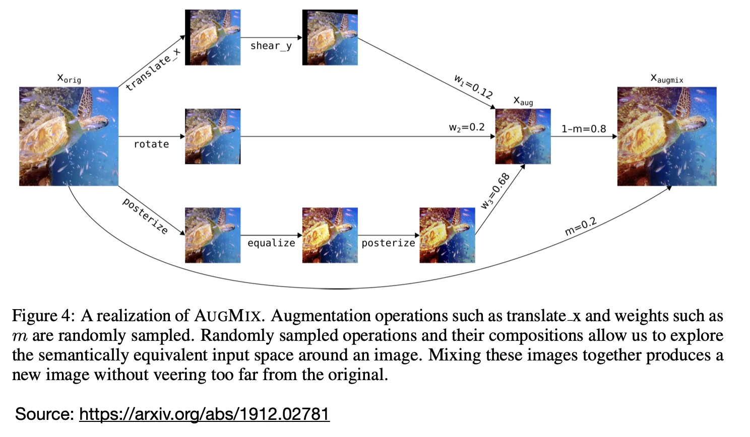
Note that in the figure above, the final image \(x_{\text{augmix}}\) is obtained by interpolating (mixing) the augmented image \(x_{\text{aug}}\) with the original image \(x_{\text{orig}}\), and \(x_{\text{aug}}\) is obtained by applying different mixing weights (\(w_1, w_2, w_3\)) as well.
To this end, the researchers optimize an overall loss that consists of two components:
\[\text{Loss}_{\text{overall}} = \text{Loss}_{\text{classification}} + \text{Loss}_{\text{consistency}}.\]The classification loss is a standard cross-entropy loss, and the consistency loss is the Jensen-Shannon divergence between the softmax output from applying the model to the original image and the softmax output from applying the model to the augmented images.
(The Jensen-Shannon divergence is a symmetric version of the Kullback-Leibler divergence for measuring the difference between two probability distributions. The Kullback-Leibler divergence itself is the same as cross-entropy minus the self-entropy term.)
TrivialAugment
TrivialAugment is a minimalist approach that only applies one augmentation per image. In contrast to AutoAugment or AugMix, this is not a learned procedure.
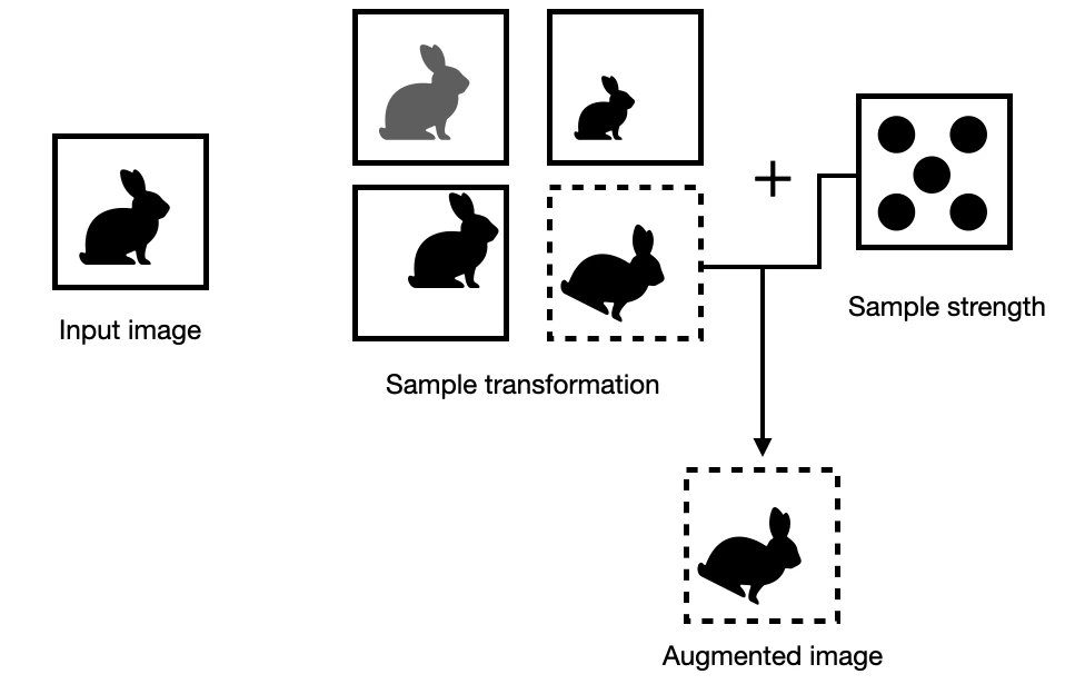
On the surface, TrivialAugment appears to be a special case of RandAugment. However, RandAugment may apply more than one image transformation per image. In contrast, TrivialAugment strictly applies only a single augmentation. Also, RandAugment uses a fixed augmentation strength per image (the strength is a hyperparameter and is applied to each image in the dataset). In contrast, TrivialAugment samples the strength randomly for each individual image.
Read Next
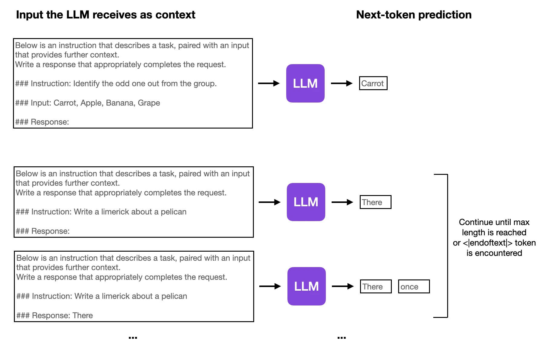 Optimizing LLMs From a Dataset Perspective
Practical guide to improving LLM finetuning with better instruction datasets, covering data curation, prompt-output pairs, synthetic data, and experiment i
Optimizing LLMs From a Dataset Perspective
Practical guide to improving LLM finetuning with better instruction datasets, covering data curation, prompt-output pairs, synthetic data, and experiment i
 The NeurIPS 2023 LLM Efficiency Challenge Starter Guide
Large language models (LLMs) offer one of the most interesting opportunities for developing more efficient training methods. A few weeks ago, the NeurIPS..
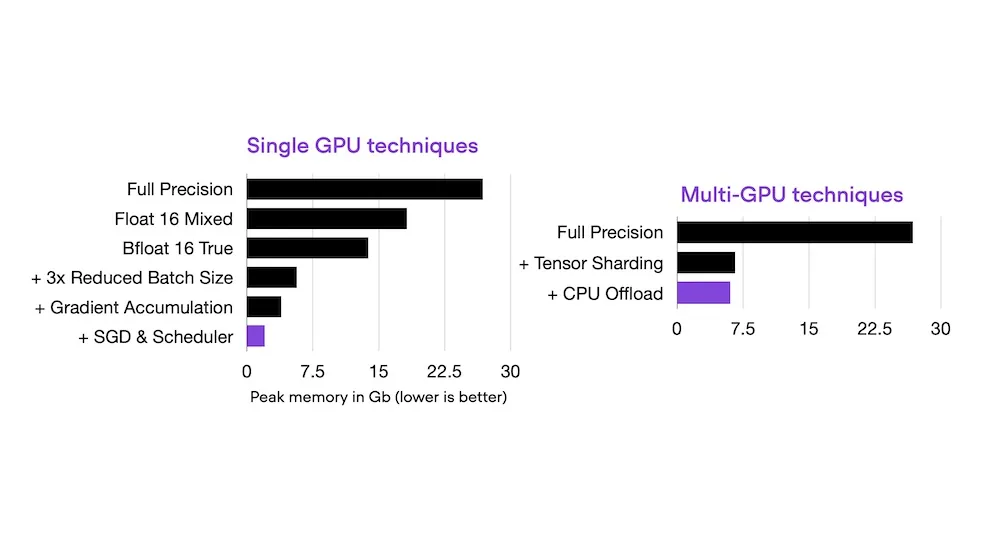
Optimizing Memory Usage for Training LLMs and Vision Transformers in PyTorch
Peak memory consumption is a common bottleneck when training deep learning models such as vision transformers and LLMs. This article provides a series of..
The NeurIPS 2023 LLM Efficiency Challenge Starter Guide
Large language models (LLMs) offer one of the most interesting opportunities for developing more efficient training methods. A few weeks ago, the NeurIPS..
Optimizing Memory Usage for Training LLMs and Vision Transformers in PyTorch
Peak memory consumption is a common bottleneck when training deep learning models such as vision transformers and LLMs. This article provides a series of..

If you read the book and have a few minutes to spare, I'd really appreciate a brief review. It helps us authors a lot!
Your support means a great deal! Thank you!