TorchMetrics
-- How do we use it, and what's the difference between .update() and .forward()?
TorchMetrics is a really nice and convenient library that lets us compute the performance of models in an iterative fashion. It’s designed with PyTorch (and PyTorch Lightning) in mind, but it is a general-purpose library compatible with other libraries and workflows.
This iterative computation is useful if we want to track a model during iterative training or evaluation on minibatches (and optionally across on multiple GPUs). In deep learning, that’s essentially all the time. Personally, it helped me reduce a lot of my boilerplate code.
However, when using TorchMetrics, one common question is whether we should use .update() or .forward()? (And that’s also a question I certainly had when I started using it.)
While the documentation explains what’s going on when calling .forward(), it may make sense to augment the explanation with a hands-on example in this blogpost.
(PS: A Jupyter Notebook version of this blogpost can be found here.)
Computing the accuracy manually for comparison
While TorchMetrics allows us to compute much fancier things (e.g., see the confusion matrix at the bottom of my other notebook here), let’s stick to the regular classification accuracy since it is more minimalist and intuitive to compute.
Also, before we dive into TorchMetrics, let’s compute the accuracy manually to ensure we have a baseline for understanding how TorchMetrics works.
Suppose we are training a model for an epoch that consists of 10 minibatches (or batches for short). In the following code, we will simulate this via the outer for-loop (for i in range(10):).
Moreover, instead of using an actual dataset and model, let’s pretend that
-
y_true = torch.randint(low=0, high=2, size=(10,))is a tensor with the ground truth labels for our minibatch. It consists ten 0’s and 1’s.
(E.g., it is similar to something like
torch.tensor([0, 1, 1, 0, 1, 0, 1, 1, 0, 1]).) -
y_pred = torch.randint(low=0, high=2, size=(10,))are the predicted class labels for our minibatch. It’s a tensor consisting of ten 0’s and 1’s similar toy_true.
Via torch.manual_seed(123), we ensure that the code is reproducible and gives us exactly the same results each time we execute the following code cell:
In:
import torch


torch.manual_seed(123)

all_true, all_pred = [], []

for i in range(10):
    y_true = torch.randint(low=0, high=2, size=(10,))
    y_pred = torch.randint(low=0, high=2, size=(10,))
    all_true.append(y_true)
    all_pred.append(y_pred)

correct_pred = (torch.cat(all_true) == torch.cat(all_pred)).float()

acc = torch.mean(correct_pred)
print('Overall accuracy:', acc)
Out:
Overall accuracy: tensor(0.5600)
So, what we have done above is we collected all the true class labels all_true, and all_pred. Then, we computed the number of correct predictions (the number of times the true and the predicted labels match) and assigned this number to correct_pred. Finally, we computed the average number of correct predictions, which is our accuracy.
If we work with large datasets, it would be wasteful to accumulate all the labels via all_true and all_pred (and, in the worst case, we could exceed the GPU memory). A smarter way is to count the number of correct predictions and then divide that number by the total number of training examples as shown below:
In:
torch.manual_seed(123)

num = 0
correct = 0.

for i in range(10):
    y_true = torch.randint(low=0, high=2, size=(10,))
    y_pred = torch.randint(low=0, high=2, size=(10,))
    correct += (y_true == y_pred).float().sum()
    num += y_true.numel()

acc = correct / num
print('Overall accuracy:', acc)
Out:
Overall accuracy: tensor(0.5600)
Using TorchMetrics
So, TorchMetrics allows us to do what we have done in the previous section; that is, iteratively computing a metric.
The general steps are as follows:
- We initialize a metric we want to compute (here: accuracy).
- We call
.update()during the training loop. - Finally, we call
.compute()to get the final accuracy value when we are done.
Let’s take a look at what this looks like in code:
In:
from torchmetrics.classification import Accuracy


train_acc = Accuracy()
torch.manual_seed(123)

for i in range(10):

    y_true = torch.randint(low=0, high=2, size=(10,))
    y_pred = torch.randint(low=0, high=2, size=(10,))

    abc = train_acc.update(y_true, y_pred)
    print('Batch accuracy:', abc)

print('Overall accuracy:', train_acc.compute())
Out:
Batch accuracy: None
Batch accuracy: None
Batch accuracy: None
Batch accuracy: None
Batch accuracy: None
Batch accuracy: None
Batch accuracy: None
Batch accuracy: None
Batch accuracy: None
Batch accuracy: None
Overall accuracy: tensor(0.5600)
Notice that the overall accuracy is the same that we got from computing it manually in the previous section. For reference, we also printed the accuracy for each minibatch; however, there is nothing interesting here because it’s always None. The following code example will make it clear why we did that.
So, in the following code example, we make a small modification to the training loop. Now, we are calling train_acc.forward() (or, to be more precise, the equivalent shortcut train_acc()) instead of train_acc.update(). The .forward() call does a bunch of things under the hood, which we will talk about later. For now, let’s just inspect the results:
In:
train_acc = Accuracy()

torch.manual_seed(123)
for i in range(10):

    y_true = torch.randint(low=0, high=2, size=(10,))
    y_pred = torch.randint(low=0, high=2, size=(10,))

    # the following two lines are equivalent:
    # abc = train_acc.forward(y_true, y_pred)
    abc = train_acc(y_true, pred)

    print('Batch accuracy:', abc)

print('Overall accuracy:', train_acc.compute())
Out:
Batch accuracy: tensor(0.7000)
Batch accuracy: tensor(0.7000)
Batch accuracy: tensor(0.5000)
Batch accuracy: tensor(0.6000)
Batch accuracy: tensor(0.4000)
Batch accuracy: tensor(0.4000)
Batch accuracy: tensor(0.6000)
Batch accuracy: tensor(0.6000)
Batch accuracy: tensor(0.5000)
Batch accuracy: tensor(0.6000)
Overall accuracy: tensor(0.5600)
As we can see, the overall accuracy is the same as before (as we would expect 😊). However, we now also have the intermediate results: the batch accuracies. The batch accuracy refers to the accuracy of the given minibatch. For reference, below is how it looks like if we compute it manually:
In:
torch.manual_seed(123)

num = 0
correct = 0.

for i in range(10):
    y_true = torch.randint(low=0, high=2, size=(10,))
    y_pred = torch.randint(low=0, high=2, size=(10,))

    correct_batch = (y_true == pred).float().sum()
    correct += correct_batch
    num += y_true.numel()

    abc = correct_batch / y_true.numel()
    print('Batch accuracy:', abc)

acc = correct / num
print('Overall accuracy:', acc)
Out:
Batch accuracy: tensor(0.7000)
Batch accuracy: tensor(0.7000)
Batch accuracy: tensor(0.5000)
Batch accuracy: tensor(0.6000)
Batch accuracy: tensor(0.4000)
Batch accuracy: tensor(0.4000)
Batch accuracy: tensor(0.6000)
Batch accuracy: tensor(0.6000)
Batch accuracy: tensor(0.5000)
Batch accuracy: tensor(0.6000)
Overall accuracy: tensor(0.5600)
If we are interested in the validation set or test accuracy, this intermediate result is maybe not super useful. However, it can be handy for tracking the training set accuracy during training. Also, it is useful for things like the loss function. This way, we can plot both the intermediate loss per minibatch and the average loss per epoch with only one pass over the training set.
.update() vs .forward() – the official explanation
So, in the previous section, we saw that both .forward() and .update() do slightly different things. The .update() method is somewhat simpler: it just updates the metric. In contrast, .forward() updates the metric, but it also lets us report the metric for each individual batch update. The .forward() method is essentially a more sophisticated method that uses .update() under the hood.
Which method should we use? It depends on our use case. If we don’t care about tracking or logging the intermediate results, using .update() should suffice. However, calling .forward() is usually computationally very cheap – in the grand scheme of training deep neural networks – so it’s not harmful to default to using .forward(), either.
If you are interested in the nitty-gritty details, have a look at the following excerpt from the official documentation:
The
forward()method achieves this by combining calls toupdateandcomputein the following way:
- Calls
update()to update the global metric state (for accumulation over multiple batches)- Caches the global state.
- Calls
reset()to clear global metric state.- Calls
update()to update local metric state.- Calls
compute()to calculate metric for current batch.- Restores the global state.
This procedure has the consequence of calling the user defined
updatetwice during a singleforwardcall (one to update global statistics and one for getting the batch statistics).
Bonus: Computing the running average
The fact that there are separate .update() and .compute() methods allow us to compute the running average of a metric (rather then the metric on the single batch). To achieve this, we can include a .compute() call inside the loop:
In:
from torchmetrics.classification import Accuracy


train_acc = Accuracy()
torch.manual_seed(123)

for i in range(10):

    y_true = torch.randint(low=0, high=2, size=(10,))
    y_pred = torch.randint(low=0, high=2, size=(10,))

    train_acc.update(y_true, y_pred)
    abc = train_acc.compute()
    print('Running accuracy:', abc)

print('Overall accuracy:', train_acc.compute())
Out:
Running accuracy: tensor(0.7000)
Running accuracy: tensor(0.7000)
Running accuracy: tensor(0.6333)
Running accuracy: tensor(0.6250)
Running accuracy: tensor(0.5800)
Running accuracy: tensor(0.5500)
Running accuracy: tensor(0.5571)
Running accuracy: tensor(0.5625)
Running accuracy: tensor(0.5556)
Running accuracy: tensor(0.5600)
Overall accuracy: tensor(0.5600)
The preciding code is equivalent to the following manual computation:
In:
torch.manual_seed(123)

num = 0
correct = 0.

for i in range(10):
    y_true = torch.randint(low=0, high=2, size=(10,))
    y_pred = torch.randint(low=0, high=2, size=(10,))

    correct_batch = (y_true == y_pred).float().sum()
    correct += correct_batch
    num += y_true.numel()

    abc = correct / num
    print('Running accuracy:', abc)

acc = correct / num
print('Overall accuracy:', acc)
Out:
Running accuracy: tensor(0.7000)
Running accuracy: tensor(0.7000)
Running accuracy: tensor(0.6333)
Running accuracy: tensor(0.6250)
Running accuracy: tensor(0.5800)
Running accuracy: tensor(0.5500)
Running accuracy: tensor(0.5571)
Running accuracy: tensor(0.5625)
Running accuracy: tensor(0.5556)
Running accuracy: tensor(0.5600)
Overall accuracy: tensor(0.5600)
Read Next
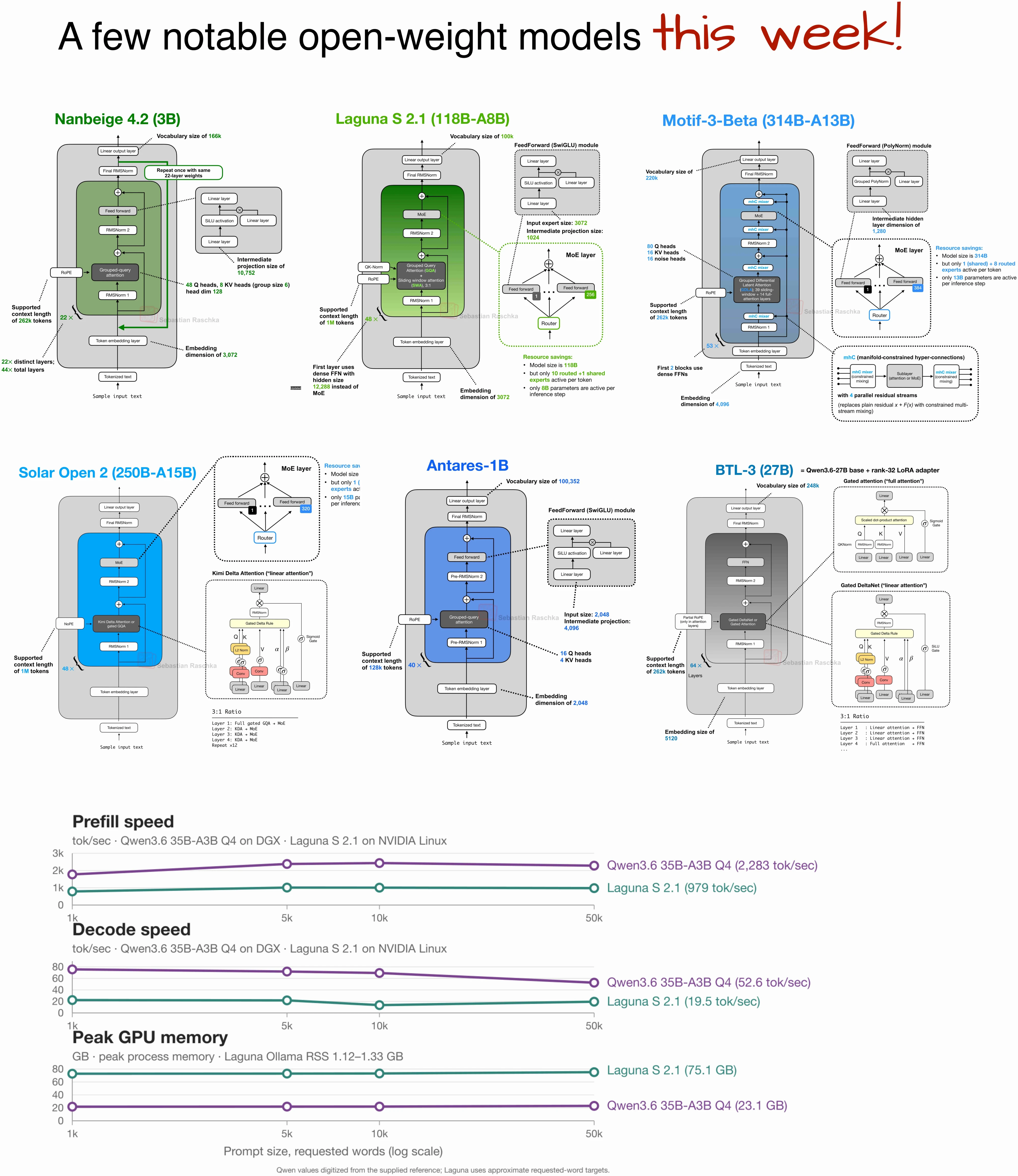 A Few Notable Open-Weight Models This Week
Short note on the architectures of six new open-weight models, including Nanbeige 4.2, Laguna S 2.1, Motif-3-Beta, Solar Open 2, Antares 1B, and BTL-3.
A Few Notable Open-Weight Models This Week
Short note on the architectures of six new open-weight models, including Nanbeige 4.2, Laguna S 2.1, Motif-3-Beta, Solar Open 2, Antares 1B, and BTL-3.
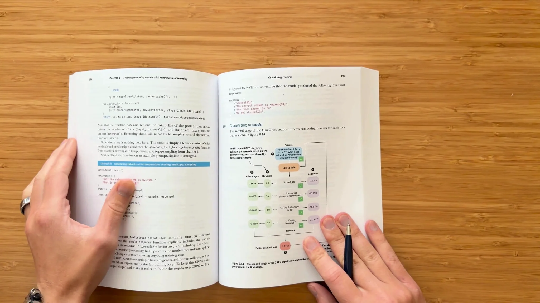 Correction for Listing 6.5 in Build a Reasoning Model From Scratch
Short correction note for the random seed in Listing 6.5 on page 198 of Build a Reasoning Model From Scratch.
Correction for Listing 6.5 in Build a Reasoning Model From Scratch
Short correction note for the random seed in Listing 6.5 on page 198 of Build a Reasoning Model From Scratch.
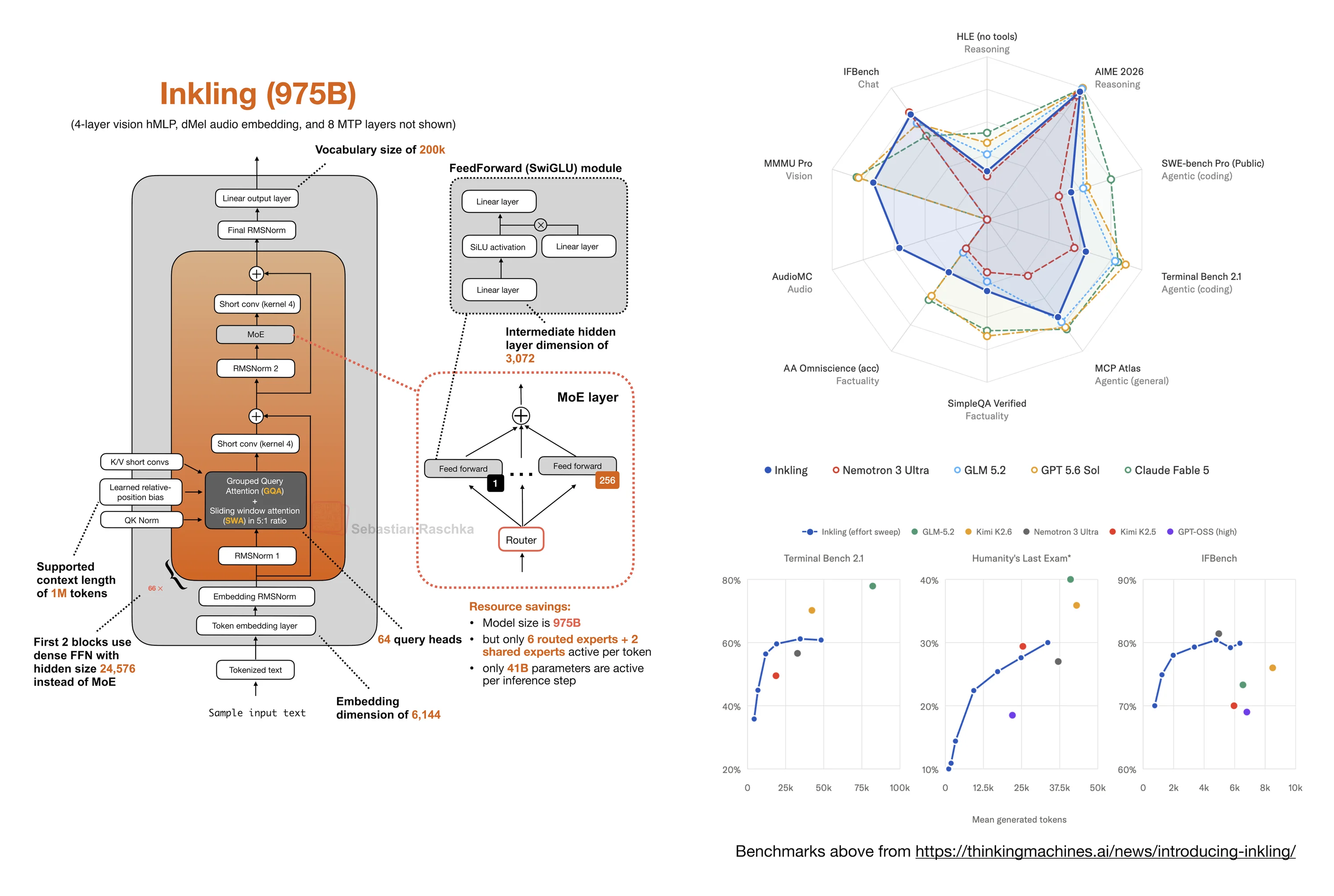 Inkling: A New Open-Weight 975B MoE with a Few Surprises
Short note on Thinking Machines Lab's 975B Inkling model, including benchmarks, sparse MoE design, short convolutions, RMSNorm, and position bias.
Inkling: A New Open-Weight 975B MoE with a Few Surprises
Short note on Thinking Machines Lab's 975B Inkling model, including benchmarks, sparse MoE design, short convolutions, RMSNorm, and position bias.

If you read the book and have a few minutes to spare, I'd really appreciate a brief review. It helps us authors a lot!
Your support means a great deal! Thank you!