Taking Datasets, DataLoaders, and PyTorch’s New DataPipes for a Spin
The PyTorch team recently announced TorchData, a prototype library focused on implementing composable and reusable data loading utilities for PyTorch. In particular, the TorchData library is centered around DataPipes, which are meant to be a DataLoader-compatible replacement for the existing Dataset class.
I honestly don’t dislike PyTorch’s existing Dataset and DataLoader utilities, but I also love trying new things. So, in this article, I try to provide some concise examples along with some thoughts after taking the new DataPipe API for a spin.
You can find the complementary code files on GitHub here. The code was originally developed and tested with:
Python version: 3.8.13

torch: 1.11.0
torchdata: 0.3.0
- Data Loading? What’s the Big Deal?
- Setting the Stage
- Dataset & DataLoader
- Creating Datasets with ImageFolder
- Introduction to DataPipes
- DataPipes for Datasets With Images and CSVs
- Conclusions
Data Loading? What’s the Big Deal?
Who doesn’t want deep learning models to train faster? Of course, many factors influence the training time, such as the model architecture, the number of data points, batch size, GPU, storage drive, and the list goes on and on.
However, we want to ensure that data loading doesn’t become a bottleneck, especially if we buy or rent that fancy GPU. In other words, we want to ensure that the GPU never has to wait for a batch of new data.
Let’s illustrate the problem with an example. Suppose we have the following PyTorch training loop setup:
for epoch in range(num_epochs):

    inputs = []
    # prepare next minibatch
    for f in filename_minibatch:
        img = Image.open(os.path.join(img_dir, f))
        img_tensor = o_tensor(img).to('cuda')
        inputs.append(img_tensor)
    inputs = torch.cat(inputs)

    # train model
    logits = model(inputs)
    ...
    loss.backward()
    optimizer.step()
This is bad! Why? Because training and data loading happen sequentially in the same for-loop. Each time we load the next minibatch, the model and GPU are sitting idle.
The code above creates a data bottleneck where the model (and GPU) are waiting for the next batch, which is illustrated in the following figure:
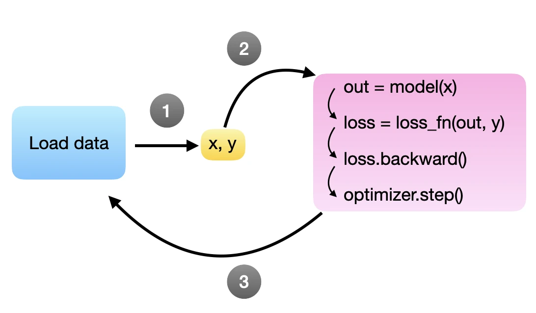
In an ideal world, we want the model to process the next minibatch immediately after the backward call and parameter update (via .step()). Or in other words, the goal is to have the next minibatch ready as soon as the model is ready, so we want to keep loading the minibatches in the background while the model is training. Unfortunately, since Python has a global interpreter lock (GIL) that only allows it to run a single process by default, we would have to write a complicated workaround.
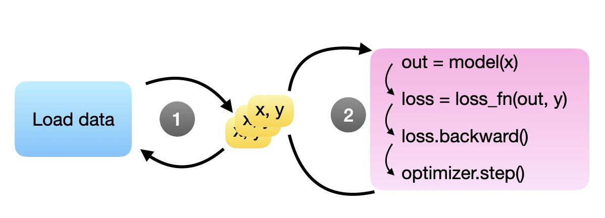
Thankfully, someone has already solved this problem for us: we can use PyTorch’s DataLoader that does precisely that. The DataLoader lets us specify the number of background processes for loading the next minibatches, so we don’t stall the GPU. This is illustrated in the figure below, where steps 1 and 2 are independent processes running in parallel. Here, the idea is that multiple training examples (“x, y”’s) are available at all times for the model to grab for the next round – in theory, one would already be sufficient.
Commonly, we use the Dataset class together with the DataLoader class. We define a Dataset instance how the data files are opened, and the DataLoader helps with
- shuffling the data,
- collating the data into minibatches,
- using multiple processes to prepare the minibatches in the background,
- and more.
Now, one goal of DataPipes is to provide some reusable components for building Datasets more flexibly. Another goal is to simplify the DataLoader. Currently, the DataLoader has a relatively complex logic to do many things. Some of this functionality will be encoded in the DataPipe itself, which opens the way for a new DataLoader2 in future versions of PyTorch.
(Note that as of this writing, there is already a prototype of DataLoader2 in the TorchData library, which you can find here – thanks to Elijah Rippeth for pointing it out. However, currently the main way to use DataPipes is to combine it with the existing DataLoader. Also, the PyTorch team aims to keep the original Dataset and DataLoader, so you don’t have to worry about adopting DataPipes right away.).
In this article, we will first look at how we currently use Dataset with DataLoader. Then, we will see how we can compose DataPipes that, together with DataLoader, reproduce this behavior.
Setting the Stage
In the following sections, we will look at some hands-on examples of implementing Datasets, DataLoaders, and DataPipes. We will use the boring MNIST dataset to keep it simple. Of course, an MNIST dataset is already included in PyTorch, but using that would be cheating. Instead, we will use a version of the MNIST dataset organized as individual PNG image files. This is to mimic an arbitrary real-world deep learning project where you have a bunch of files organized in various folders.
To keep this article focused on the essentials, we are not going through the code for obtaining the dataset. However, if you want to download the dataset to your computer to play around with it, you can run the 0_download-and-prep-data.ipynb Jupyter notebook. After running the code, there should be a mnist-png folder that contains two subfolders: train and test. Each of these subfolders consists of 10 more subfolders. These subfolders with the numbers 0-9 correspond to the class labels. Inside each folder are the actual PNG files:
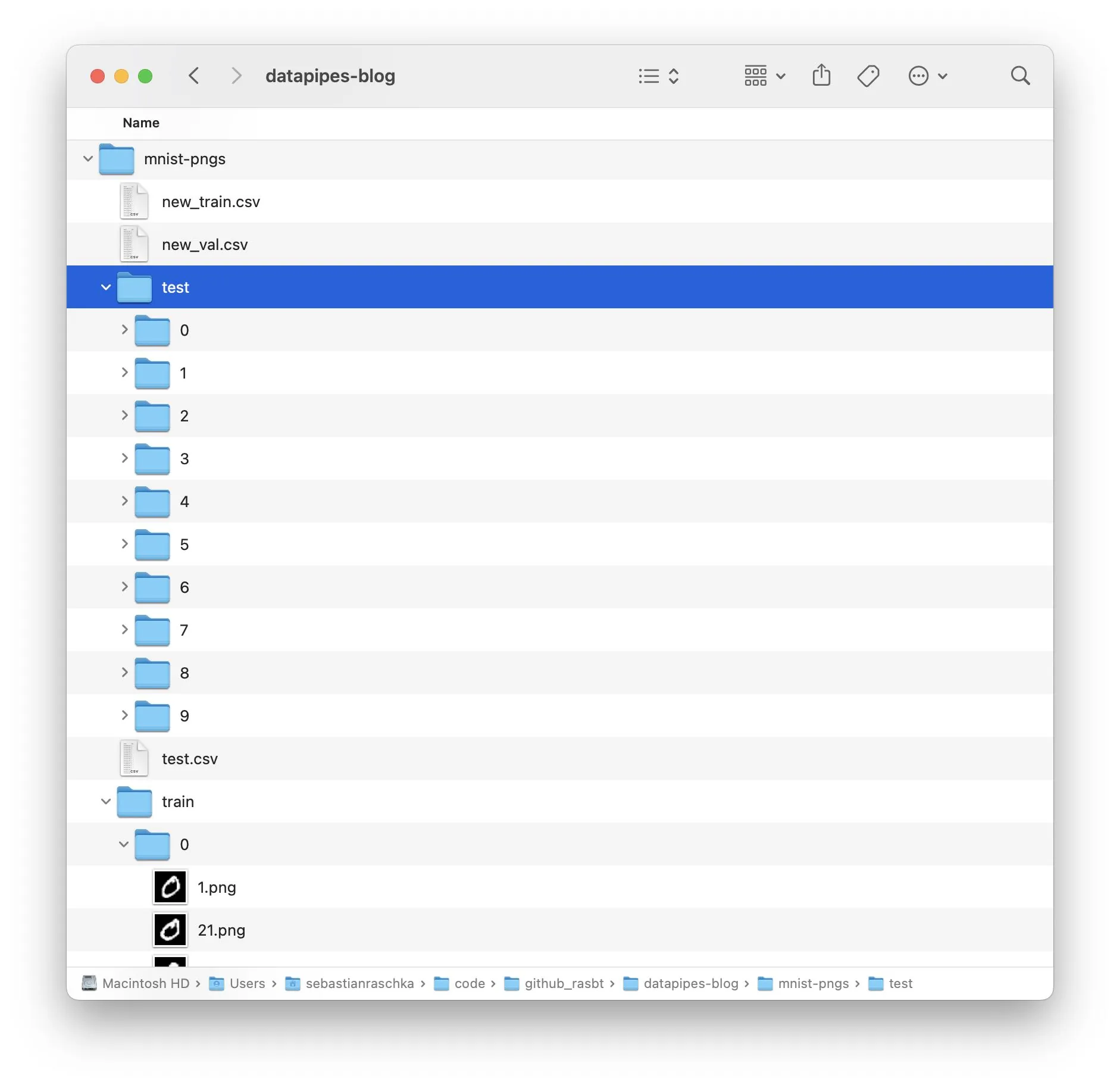
There should be 50k PNGs for training and 10k PNGs for testing.
In addition to the subfolders and PNG files, there are also three CSV files: test.csv, new_train.csv, and new_val.csv. Those contain the individual file paths and labels for the three data subsets. Shown below are the first five lines of the training and validation set CSV files for illustration purposes:
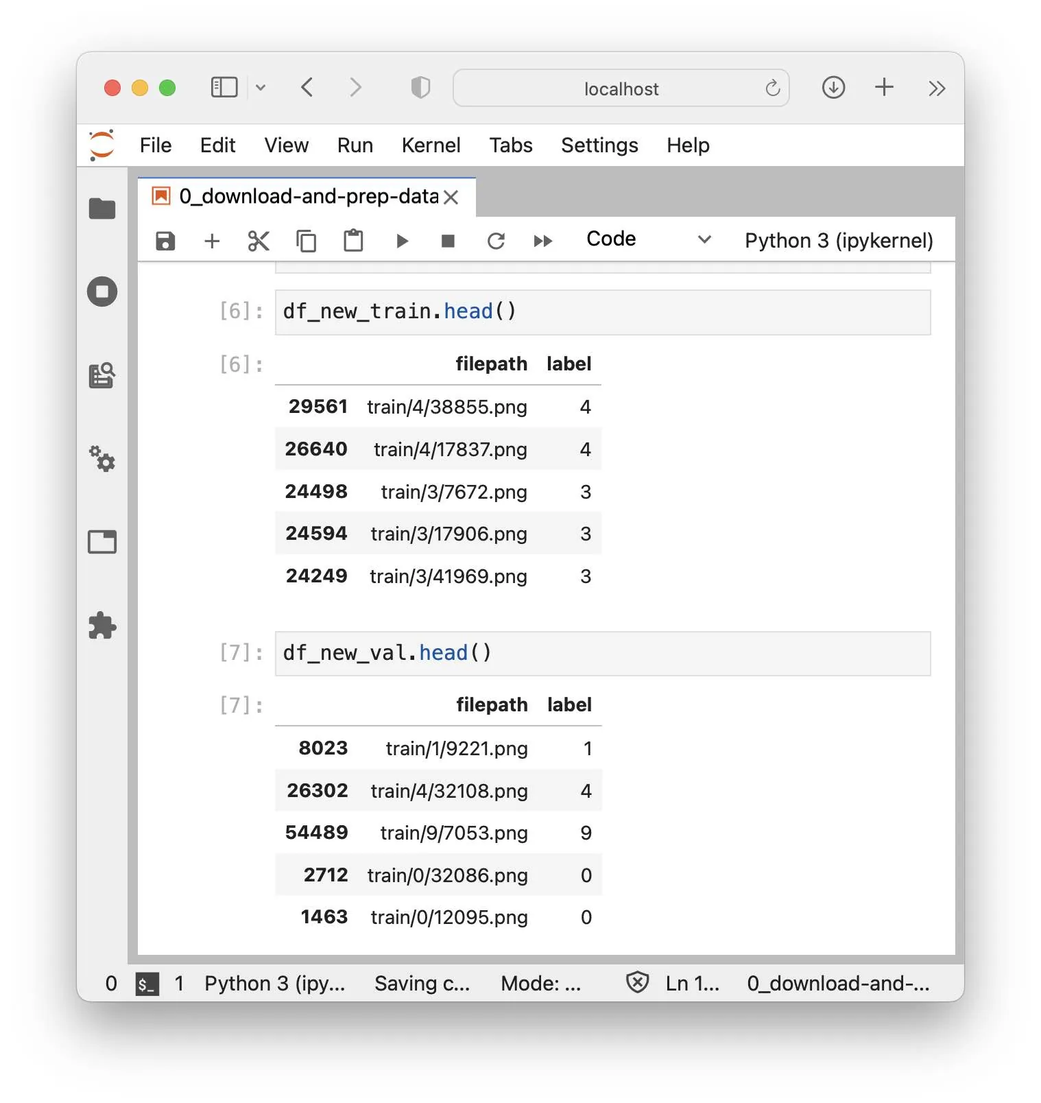
Please note that the MNIST dataset does not have a dedicated validation set folder. To generate the new_train.csv and new_val.csv, a CSV file with 50k training set images was split into 45k images for training and 5k images for validation, which is why the file paths of the validation set CSV also contain train in the filepath name.
Dataset & DataLoader
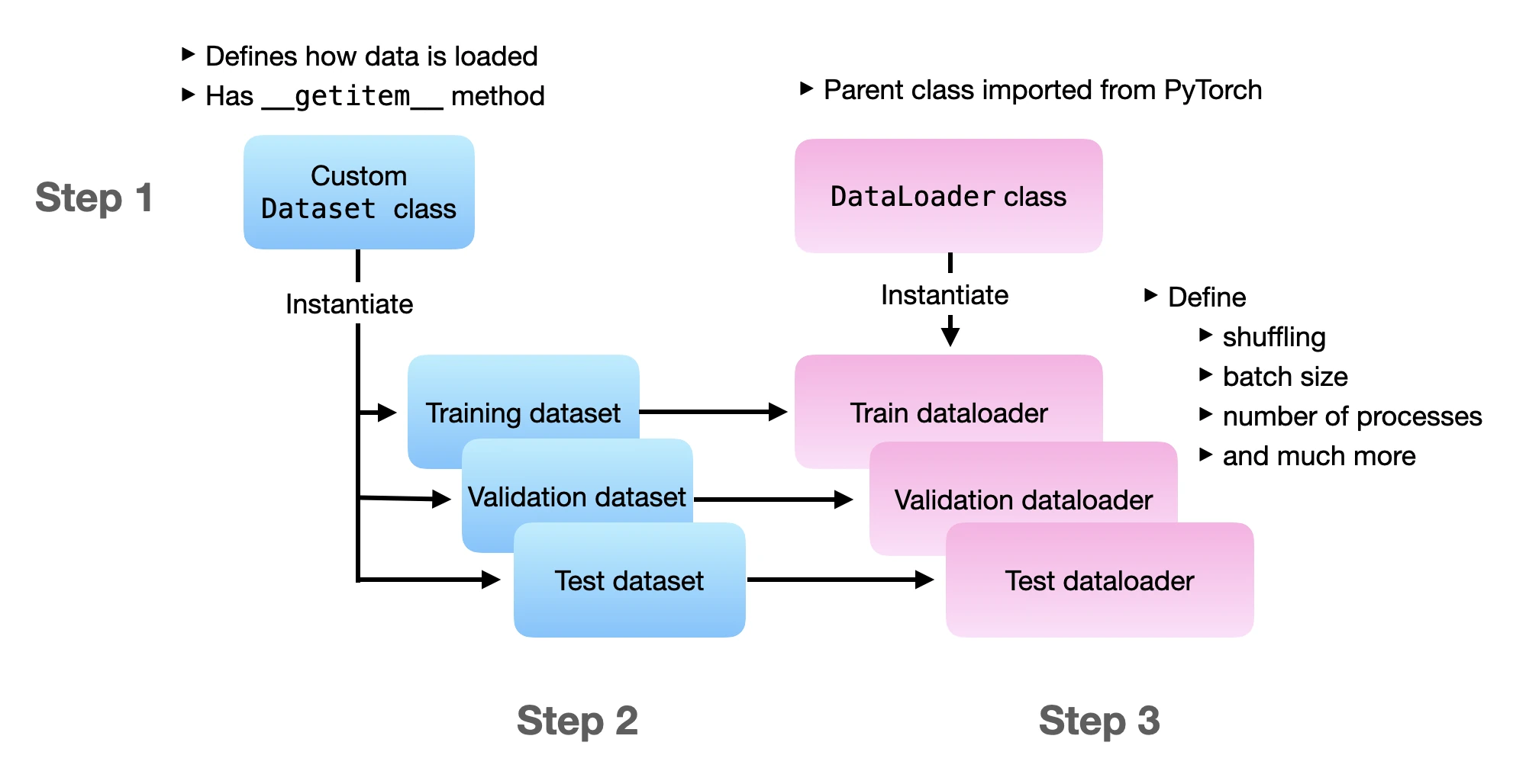
In this section, we are loading the Dataset and DataLoader the traditional way. In step 1, we define the datasets that contain all the file loading logic. In step 2, we instantiate dataset objects for the training, validation, and test set. In step 3, we are instantiating the data loaders. And in step 4, we are doing a test iteration to ensure that the data loaders work.
Before we dive in, the following figure illustrates the overall flow of the three main steps:
If you want to run the following code yourself, I recommend referring to the self-contained 1_dataset-csv.py file from this article’s accompanying GitHub repo.
Step 1: Defining a Custom Dataset
In this section, we are defining a custom Dataset class for loading training examples. A dataset typically consists of three methods.
-
__init__: The constructor that contains or calls the main dataset setup code. -
__getitem__: A method that specifies how to load a single data instance. -
__len__: A method that returns the total number of data instances.
Let’s have a look at the following MyDataset class that subclasses from PyTorch’s Dataset:
import os
import pandas as pd
from PIL import Image
from torch.utils.data import Dataset


class MyDataset(Dataset):
    def __init__(self, csv_path, img_dir, transform=None):

        df = pd.read_csv(csv_path)
        self.img_dir = img_dir
        self.transform = transform

        # based on DataFrame columns
        self.img_names = df["filepath"]
        self.labels = df["label"]

    def __getitem__(self, index):
        img = Image.open(os.path.join(self.img_dir, self.img_names[index]))

        if self.transform is not None:
            img = self.transform(img)

        label = self.labels[index]
        return img, label

    def __len__(self):
        return self.labels.shape[0]
The __init__ method contains code to open a CSV file using Pandas. It also stores the "filepath" and "label" columns as attributes so that we can refer to these in the other Dataset methods later.
The __getitem__ method takes an index argument that refers to a single data instance. If our dataset consists of 50,000 training examples, the index would be a number between 0 and 49,999. Inside the __getitem__ method, we then use the index to fetch a filename from our file path list via self.img_names[index]) and open the image via PIL. Note that the PIL image then goes through an optional transformation step – typically, this should at least be a conversion to a PyTorch tensor data type if we are using PyTorch for model training, but more on that later. Lastly, we get the corresponding label and return the “img, label” pair.
The __len__ method is relatively boring; it simply returns the length of the dataset, which we can get from the labels column, which we assigned to self.labels earlier.
In sum, our custom MyDataset class defines how we can open and return individual files. In the next section, we will instantiate custom MyDataset instances.
Step 2: Instantiating Training, Validation, and Test sets
Now that we have our custom MyDataset class, we can instantiate our datasets for the data loader. In the following code, we create separate datasets for training, validation, and testing:
train_dataset = MyDataset(
    csv_path="mnist-pngs/new_train.csv",
    img_dir="mnist-pngs/",
    transform=data_transforms["train"],
)

val_dataset = MyDataset(
    csv_path="mnist-pngs/new_val.csv",
    img_dir="mnist-pngs/",
    transform=data_transforms["test"],
)

test_dataset = MyDataset(
    csv_path="mnist-pngs/test.csv",
    img_dir="mnist-pngs/",
    transform=data_transforms["test"],
)
Note that the training set uses different transformation steps (data_transforms["train"]) than the validation and test set (data_transforms["test"]). So let’s define these transformation steps, which will clarify why that is:
from torchvision import transforms

data_transforms = {
    "train": transforms.Compose(
        [
            transforms.Resize(32),
            transforms.RandomCrop((28, 28)),
            transforms.ToTensor(),
            # normalize images to [-1, 1] range
            transforms.Normalize((0.5,), (0.5,)),
        ]
    ),
    "test": transforms.Compose(
        [
            transforms.Resize(32),
            transforms.CenterCrop((28, 28)),
            transforms.ToTensor(),
            # normalize images to [-1, 1] range
            transforms.Normalize((0.5,), (0.5,)),
        ]
    ),
}
Here, we include some data transformation (RandomCrop) in the training loader. However, we don’t want any randomness during inference, which is why the "test" transformation step uses a CenterCrop instead. (If we omit the CenterCrop in the "test" transformation, the training and test set images will have different resolutions, which is also not ideal.) Since we use the validation set as a proxy for measuring the generalization performance during training, I recommend treating it similarly to the test set.
Lastly, a short note about the ToTensor transformation: the steps of the preceding transformation, such as Resize and CenterCrop operate on the PIL images returned by the Dataset’s__getitem__ method. The ToTensor transformation converts the PIL image into a PyTorch tensor with pixel values normalized to 0 and 1. The Normalize transformation implements z-score standardization, that is, subtracting a mean value and dividing by a standard deviation: \(x' = \frac{x - \mu}{\sigma}.\)
In transforms.Normalize((0.5,), (0.5,)), the first tuple contains the mean values – one value for each color channel. Since MNIST comes in a grayscale format, it only contains one color channel. The second tuple contains the standard deviation values. We would write the transformation as transforms.Normalize((0.5, 0.5, 0.5), (0.5, 0.5, 0.5)) for an RGB image with three color channels. Note that since ToTensor outputs pixel values within a [0, 1] range, choosing \(\mu=0.5\) and \(\sigma=0.5\) results in pixels normalized to [-1, 1] – sometimes, this results in better gradient descent behavior. In practice, it is also recommended to compute and use each channel’s actual mean and standard deviation, but this is a topic for another time.
Step 3: Creating DataLoaders
Now that we instantiated the datasets in the previous step, let’s create the training, validation, and test set data loaders:
from torch.utils.data import DataLoader

train_loader = DataLoader(
    dataset=train_dataset,
    batch_size=32,
    shuffle=True,
    drop_last=True,
    transform=data_transforms["train"],
    num_workers=2,
)

val_loader = DataLoader(
    dataset=val_dataset,
    batch_size=32,
    shuffle=False,
    transform=data_transforms["test"],
    num_workers=2,
)

test_loader = DataLoader(
    dataset=test_dataset,
    batch_size=32,
    shuffle=False,
    transform=data_transforms["test"],
    num_workers=2
)
Above, we instantiated each dataloader with its corresponding dataset: train_dataset , val_dataset, and test_dataset.
We set num_workers=2 to ensure that at least two subprocesses are used to load the data in parallel using the CPU (while the GPU or another CPU is busy training the model.) MNIST images are very, very small, so num_workers=2 should be sufficient in this case. However, you may want to consider allocating more workers for datasets with larger image sizes and more extensive data processing steps.
While we don’t need to shuffle the validation and test datasets, we set shuffle=True for instantiating the training loader. This will ensure that the training examples are shuffled in each epoch. The drop_last=True setting will drop the last batch in each epoch if the dataset is not evenly divisible by the batch size. For example, if we have a dataset with 45,000 training examples and a batch size of 32, the last batch would contain only \(45,000 - 1,406 \times 32 = 8\) examples, and sometimes these small batches can lead to noisy gradient updates, which is why I recommend using drop_last=True for the training loader.
Note that the DataLoader has many additional settings, including pin_memory, persistent_workers, and more. I encourage you to check out the official API documentation.
Step 4: Trying the DataLoaders
Finally, let’s see whether our implementation works by iterating through the first 3 minibatches:
    num_epochs = 1
    for epoch in range(num_epochs):

        for batch_idx, (x, y) in enumerate(train_loader):
            if batch_idx >= 3:
                break
            print(" Batch index:", batch_idx, end="")
            print(" | Batch size:", y.shape[0], end="")
            print(" | x shape:", x.shape, end="")
            print(" | y shape:", y.shape)

    print("Labels from current batch:", y)
The code above should print the following code (however, note that the labels may differ based on your random seed setting):
 Batch index: 0 | Batch size: 32 | x shape: torch.Size([32, 1, 28, 28]) | y shape: torch.Size([32])
 Batch index: 1 | Batch size: 32 | x shape: torch.Size([32, 1, 28, 28]) | y shape: torch.Size([32])
 Batch index: 2 | Batch size: 32 | x shape: torch.Size([32, 1, 28, 28]) | y shape: torch.Size([32])
Labels from current batch: tensor([5, 1, 1, 1, 8, 3, 1, 1, 5, 8, 8, 6, 4, 4, 8, 5, 8, 5, 5, 0, 6, 5, 8, 9,
        4, 9, 6, 9, 0, 8, 5, 8])
So far, so good; everything seems to work as intended.
The “Dataset+CSV” file approach above is a general solution for most fixed-size datasets. However, suppose you are working with an image dataset consisting of individual image files organized in subfolders (such as the MNIST dataset above). In that case, there is a more convenient way of loading the dataset, which we will discuss in the next section.
Creating Datasets with ImageFolder
Using ImageFolder can make dataset loading much more convenient when we work with image folder hierarchies. Let’s see how that works.
So, instead of defining our custom dataset (as shown in the previous Step 1), we can simply use ImageFolder to create our datasets from the folder hierarchy. Here, the subfolders are the class labels:
<img src=”/images/blog/2022/datapipes/image-folder-2.jpg” width=500 =”MNIST dataset subfolders.”>
The code is as follows:
from torchvision.datasets import ImageFolder

train_dataset = ImageFolder(
    root="mnist-pngs/train",
    transform=data_transforms["train"]
)

test_dataset = ImageFolder(
    root="mnist-pngs/test",
    transform=data_transforms["test"]
)
But what about the validation set? We can use the random_split function to create a validation subset from the training dataset:
from torch.utils.data.dataset import random_split

train_dataset, val_dataset = random_split(
    train_dataset,
    lengths=[55000, 5000]
)
Then, we can reuse the exact same the code from Step 3 and 4 above.
Check out the 2_imagefolder.py file for a self-contained example.
A potential shortcoming of this approach
Before we move on to DataPipes, can you spot the one shortcoming of this approach, though? Compared to our custom Dataset approach, the ImageFolder approach above doesn’t allow us to specify a custom transform method for the validation set. We end up using the training set transformations (including the random dataset augmentation). While this is not the end of the world, it’s also not ideal. (To circumvent this problem in practice, we could create a separate validation set folder.)
Introduction to DataPipes
Now that we understand how Dataset and DataLoader work (together), let’s get to the interesting part, the new DataPipes.
Along with the PyTorch 1.11 release, the PyTorch team announced a beta version of TorchData. TorchData is a Python library that contains new data loading utilities for PyTorch. In a nutshell, TorchData is centered around so-called data pipes and reusable data components.
The TorchData team aims to replace both the Dataset and DataLoader classes eventually. Why? Because sometimes, it can be tedious to create a custom Dataset for different use cases. Building a Dataset from a set of well-optimized components may be more efficient. Also, DataLoaders are overloaded with features, and one goal behind DataPipes is to outsource that functionality into the DataPipe components.
Today, a DataPipe is compatible with the existing DataLoader and functions as a drop-in replacement for Dataset. However, in the future, the PyTorch team may develop a leaner DataLoader2 specifically for DataPipes.
The illustration below illustrates the relationship between DataPipes and DataLoader:
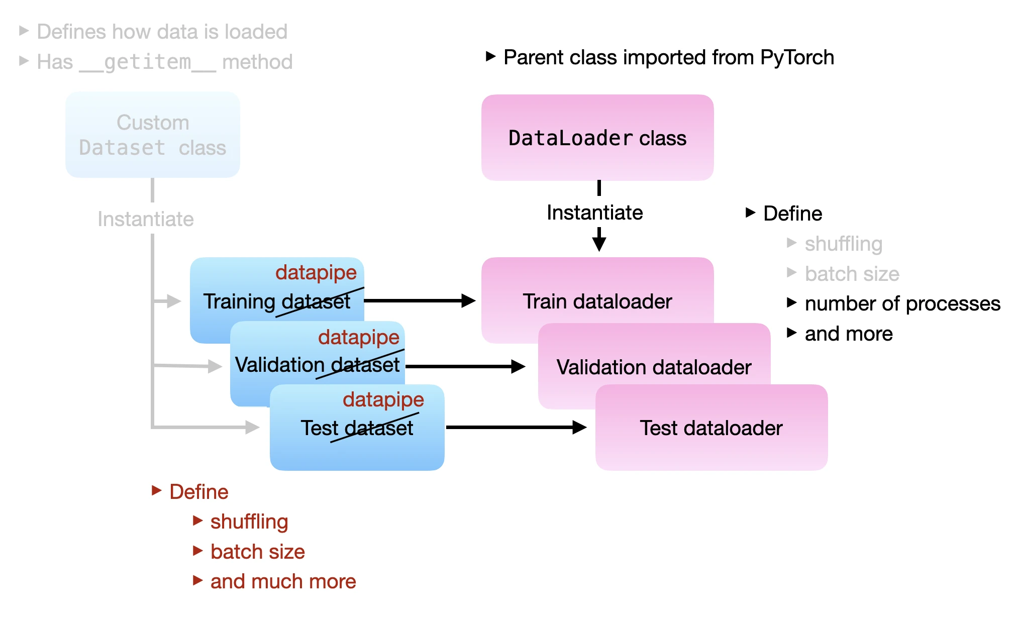
Again, the key idea is that we can construct each DataPipe (train data pipe, validation data pipe, and test data pipe) by chaining individual DataPipe components. The code examples in the following sections will make that more clear.
Class Constructors and Functional Forms
Most DataPipes can be used via their class constructor or functional form, which the PyTorch team recommends. The functional form is essentially a method call. For example, consider the following example where we use the class constructor to instantiate a new data pipe for file opening. Then, we chain a CSV parser to is using the CSVParser class constructor:
new_dp = dp.iter.FileOpener([csv_file])
new_dp = dp.iter.CSVParser(new_dp, skip_lines=1)
# returns tuples like ('train/0/16585.png', '0')
The functional form (which is recommended by the PyTorch team) would look as follows:
new_dp = dp.iter.FileOpener([csv_file])
new_dp = new_dp.parse_csv(skip_lines=1)
# returns tuples like ('train/0/16585.png', '0')
IterDataPipes and MapDataPipes
As of this writing there are two types of DataPipes: Iterable-style DataPipes (IterDataPipe) and Map-stype DataPipes (https://meta-pytorch.org/data/0.3/torchdata.datapipes.map.html).
IterDataPipes are centered around the __iter()__ protocol for fetching. This is commonly used for operations where we access data sequentially (rather than in random order). A common use case would be working with a data stream. However, another example of IterDataPipes is the FileOpener for example. The FileOpener opens files based on a list of file paths. I recommend scrolling through the list of IterDataPipes to get a brief overview of the types of IterDataPipes that exist.
MapDataPipes are centered around the __getitem__() and __len__() protocols we already know from the DataSet class. These are more meant for operations where we can have random access via dataset indices based on the length of the dataset. Again, I encourage you to scroll through the list of map-style DataPipes to see what types of MapDataPipes already exist.
Note that for certain functions like shuffling, there is both an IterDataPipe Shuffler and a MapDataPipe Shuffler. The iterable Shuffler operates on a buffer (so it only shuffles within a window size), whereas the map-style Shuffler does not have that restriction and considers the entire dataset for shuffling.
The shuffling for a IterDataPipe would look like as follows, where we have to specify a buffer size:
new_dp = dp.iter.FileOpener([csv_file])
...
new_dp = new_dp.shuffle(buffer_size=10,000)
new_dp = new_dp.map(open_image)
...
(Yes, there is also a .map method for IterDataPipes 🤯.)
However, we can convert an IterDataPipe to a MapDataPipe using .to_map_datapipe() so that we can shuffle globally:
new_dp = dp.iter.FileOpener([csv_file])
...
new_dp = new_dp.to_map_datapipe().shuffle(indices=np.arange(len))
new_dp = new_dp.map(open_image)
In the next section, we will discuss how this works in practice by implementing a DataPipe approach for our MNIST dataset.
DataPipes for Datasets With Images and CSVs
Now that we are familiar with the overall concept of DataPipes let’s reproduce the [Dataset & DataLoader] section where we worked with a CSV file containing the file paths for the MNIST images.
We are going to build three DataPipes: one for training, validation, and testing. So, let’s implement a convenience function for creating our data pipes to avoid duplicating code:
def build_data_pipe(csv_file, transform, len=1000, batch_size=32):
    new_dp = dp.iter.FileOpener([csv_file])

    new_dp = new_dp.parse_csv(skip_lines=1)
    # returns tuples like ('train/0/16585.png', '0')

    new_dp = new_dp.map(create_path_label_pair)
    # returns tuples like ('mnist-pngs/train/0/16585.png', 0)

    if transform == "train":
        new_dp = new_dp.shuffle(buffer_size=len)

    new_dp = new_dp.sharding_filter()
    # important to use sharding_filter after (not before) shuffling

    new_dp = new_dp.map(open_image)

    if transform == "train":
        new_dp = new_dp.map(apply_train_transforms)
        new_dp = new_dp.batch(batch_size=batch_size, drop_last=True)

    elif transform == "test":
        new_dp = new_dp.map(apply_test_transforms)
        new_dp = new_dp.batch(batch_size=batch_size, drop_last=False)

    else:
        raise ValueError("Invalid transform argument.")

    new_dp = new_dp.map(default_collate)
    return new_dp
In the code above, you can now see the chaining aspect of DataPipes in action. We start with a file opener IterDataPipe and add several components to it using the functional form discussed earlier.
You may also notice that there are certain variables that we have not defined, yet: create_path_label_pair, open image, apply_train_transforms , apply_test_transforms, and default_collate. These are functions we use in conjunction with .map() that we will define below:
def create_path_label_pair(inputs):
    img_path, label = inputs
    img_path = os.path.join(IMG_ROOT, img_path)
    label = int(label)
    return img_path, label


def open_image(inputs):
    img_path, label = inputs
    img = Image.open(img_path)
    return img, label


def apply_train_transforms(inputs):
    x, y = inputs
    return DATA_TRANSFORMS["train"](x), y


def apply_test_transforms(inputs):
    x, y = inputs
    return DATA_TRANSFORMS["test"](x), y
(DATA_TRANSFORMS is a global variable workaround because .map() cannot receive additional arguments at the moment. I recommend looking at the whole 3_datapipes-csv.py file for context.)
Now, using our build_data_pipe utility function, we can construct our three DataPipes:
train_dp = build_data_pipe(
    csv_file="mnist-pngs/new_train.csv", transform="train", len=45000, batch_size=32
)

val_dp = build_data_pipe(
    csv_file="mnist-pngs/new_val.csv", transform="test", batch_size=32
)

test_dp = build_data_pipe(
    csv_file="mnist-pngs/test.csv", transform="test", batch_size=32
)
Note that the dataset is relatively small, so we can use the entire length of the training set for shuffling. Notice also that both the shuffling and the batch_size are now defined inside the DataPipe rather than inside DataLoader. This is one of the many things that can enable the development of a simpler DataLoader2 in the future.
Now that we have our DataPipes defined, we can use them as a drop-in replacement for Dataset in the DataLoader:
from torch.utils.data.backward_compatibility import worker_init_fn


train_loader = DataLoader(
    dataset=train_dp, shuffle=True, num_workers=2, worker_init_fn)

val_loader = DataLoader(
    dataset=val_dp, shuffle=False, num_workers=2, worker_init_fn)

test_loader = DataLoader(
    dataset=test_dp, shuffle=False, num_workers=2, worker_init_fn)
(If you are curious about the worker_init_fn and shuffling argument in the DataLoader, please stay tuned for the Known Caveats section below.)
Now, similar to before, we can give our data loading pipeline a try with the following code
    num_epochs = 1
    for epoch in range(num_epochs):

        for batch_idx, (x, y) in enumerate(train_loader):
            if batch_idx >= 3:
                break

            # collate added an extra dimension
            x, y = x[0], y[0]
            print(" Batch index:", batch_idx, end="")
            print(" | Batch size:", y.shape[0], end="")
            print(" | x shape:", x.shape, end="")
            print(" | y shape:", y.shape)

    print("Labels from current batch:", y)
This should print the following if everything is working correctly:
 Batch index: 0 | Batch size: 32 | x shape: torch.Size([32, 1, 28, 28]) | y shape: torch.Size([32])
 Batch index: 1 | Batch size: 32 | x shape: torch.Size([32, 1, 28, 28]) | y shape: torch.Size([32])
 Batch index: 2 | Batch size: 32 | x shape: torch.Size([32, 1, 28, 28]) | y shape: torch.Size([32])
Labels from current batch: tensor([[1, 1, 7, 8, 3, 6, 6, 5, 1, 2, 4, 9, 4, 5, 1, 5, 1, 9, 4, 0, 4, 5, 1, 9,
         6, 8, 0, 0, 9, 0, 5, 4]])
Known Caveats
Multiple Processes
There are currently a few caveats worth mentioning (thanks to Nicolas Hug for pointing these out).
First, note that we used a ShardingFilter in the previous build_data_pipe function:
...
new_dp = new_dp.sharding_filter()
...
As of this writing, this is a necessary workaround to avoid data duplication when we use more than 1 worker. For example, consider the following example where we iterate over numbers in the range 0-4:
In:
from torchdata.datapipes.iter import IterableWrapper

dp = IterableWrapper(range(5))
list(DataLoader(dp, num_workers=1))
Out:
[tensor([0]),
 tensor([1]),
 tensor([2]),
 tensor([3]),
 tensor([4])]
In the code example above, the output looks like as expected. However, notice the data duplication issue if we switch to 2 workers:
In:
list(DataLoader(dp, num_workers=2))
Out:
[tensor([0]),
 tensor([0]),
 tensor([1]),
 tensor([1]),
 tensor([2]),
 tensor([2]),
 tensor([3]),
 tensor([3]),
 tensor([4]),
 tensor([4])]
To avoid this issue, we can use the .sharding_filter as workaround with a backwards compatible worker initialization function (work_init_fn):
In:
from torch.utils.data.backward_compatibility import worker_init_fn

dp = IterableWrapper(range(5))
dp = dp.sharding_filter()
list(DataLoader(dp, num_workers=2, worker_init_fn=worker_init_fn))
Out:
[tensor([0]),
 tensor([1]),
 tensor([2]),
 tensor([3]),
 tensor([4])]
Shuffling
Also, notice that even if we add a shuffling operation to our data pipeline, the data will not be shuffled by default:
In:
dp = IterableWrapper(range(5))
dp = dp.shuffle()
dp = dp.sharding_filter()
list(DataLoader(dp, num_workers=2, worker_init_fn=worker_init_fn))
Out:
[tensor([0]),
 tensor([1]),
 tensor([2]),
 tensor([3]),
 tensor([4])]
It is important to place the sharding filter after the shuffling to ensure that the data is shuffled properly.
In order to shuffle in PyTorch 1.11, we also have to enable shuffling in the DataLoader as well:
In:
list(DataLoader(
    dp, num_workers=2, worker_init_fn=worker_init_fn, shuffle=True))
Out:
 tensor([2]),
 tensor([4]),
 tensor([0]),
 tensor([3]),
 tensor([2])]
(Note that there is currently a small bug where numbers may be duplicated, as we can see above. Currently, one way to avoid this is to use only 1 worker.)
Now, one might say that the shuffling is done by the DataLoader, not the DataPipe’s .shuffle. We can confirm that it’s indeed the DataPipe that is doing the shuffling by running the following code on a DataPipe without shuffler:
In:
dp = IterableWrapper(range(5))
dp = dp.sharding_filter()
list(DataLoader(
    dp, num_workers=2, worker_init_fn=worker_init_fn, shuffle=True))
Out:
[tensor([0]),
 tensor([1]),
 tensor([2]),
 tensor([3]),
 tensor([4])]
In other words, when we use a DataPipe instead of a Dataset as input to the DataLoader, the DataLoader’s shuffle argument turns into an on/off switch for the DataPipe’s shuffler.
Now, this behavior was recently addressed in the recent nightly release of PyTorch, changes the default shuffle argument in DataLoader from False to None so that shuffling is always enabled by default if a DataPiple contains a shuffler.
Conclusions
This article covered Datasets, DataLoaders, and DataPipes. The new DataPipe classes introduced by TorchData are intended as a composable drop-in replacement for the traditional Dataset class. Now that we have seen some examples, you may have many questions!
Which Is More Convenient?
Personally, for image datasets structured similarly to the MNIST example in this article, I find Datasets more convenient than DataPipes. (And the convenience of ImageFolder is hard to beat, anyway, minus the train-transform shortcoming we discussed.) However, this is maybe owed to the fact that I am still new to DataPipes, and I still need to get used to it. However, I can see that for other use cases, especially working with streaming data and so forth, DataPipes may have certain advantages. There are also many existing IterDataPipes and MapDataPipes available for reuse, which is nice.
Which Is More Performant?
Based on my quick tests, I couldn’t notice any performance difference. To be honest, I also didn’t expect any. In the DataPipes we built in this article, we still used the same functions for Image opening and data transformation. The only difference is that we can now chain these operations. However, what’s nice about DataPipes is that this now allows for easier development and sharing, which can pave the way for developing more performant pipelines.
Which Should You Use?
It is hard to recommend one over the other at this point. For standard tasks, such as the image dataset example in this article, it is probably fine to stick with Dataset and DataLoader at the moment. In the long run, it may not hurt to start adopting DataPipes, though, since they may become the dominant way for loading data in PyTorch. Also, being familiar with it allows you to build specialized data pipes for more exotic scenarios and file formats more easily when needed.
Also, please keep in mind that DataPipes are still a beta feature. If you are currently using PyTorch 1.11 and want to use DataPipes, I recommend installing the PyTorch nightly release to get the latest updates and fixes until PyTorch 1.12 is released. You can upgrade to the latest nightly release via pip (for the detailed command, see the Installer Menu on the official PyTorch website.)
Read Next
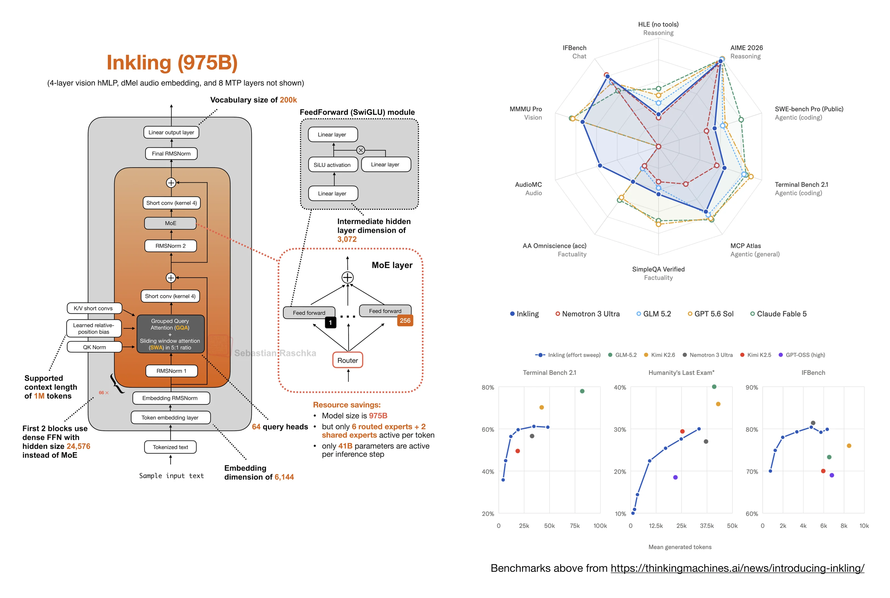 Inkling: A New Open-Weight 975B MoE with a Few Surprises
Short note on Thinking Machines Lab's 975B Inkling open-weight model, its benchmark profile, sparse MoE design, short convolutions, embedding RMSNorm, and
Inkling: A New Open-Weight 975B MoE with a Few Surprises
Short note on Thinking Machines Lab's 975B Inkling open-weight model, its benchmark profile, sparse MoE design, short convolutions, embedding RMSNorm, and
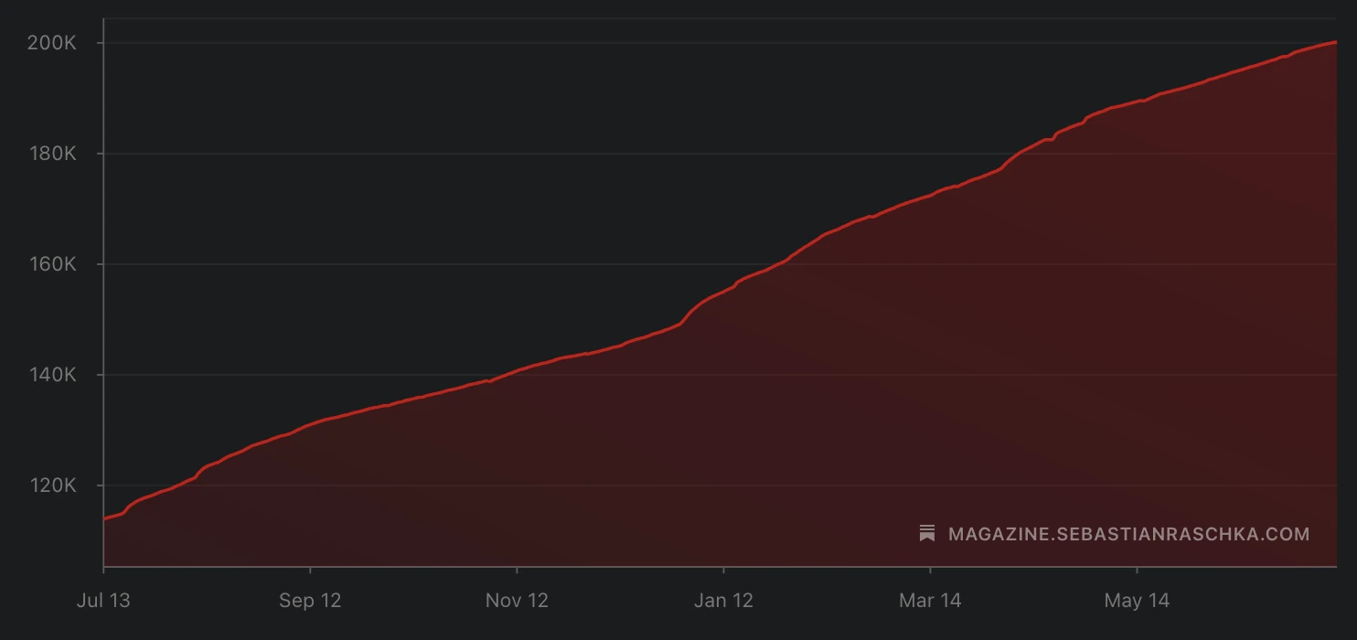 200,000 Subscribers
Short note celebrating Ahead of AI reaching 200,000 subscribers.
200,000 Subscribers
Short note celebrating Ahead of AI reaching 200,000 subscribers.
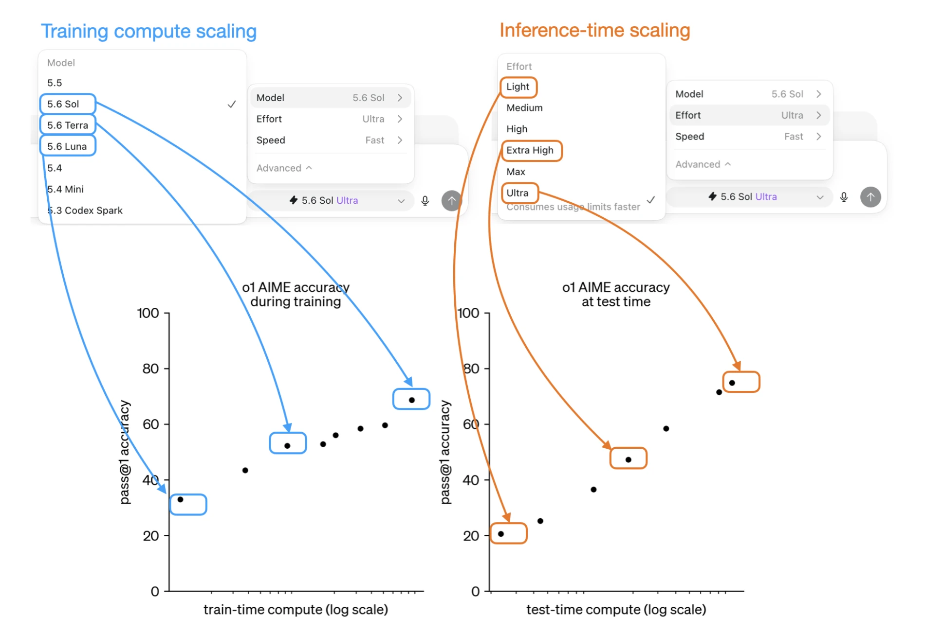 GPT 5.6 Has 72 Possible Configurations. What's A Good Default?
Short note on how GPT 5.6 model and effort choices map onto training-time and inference-time scaling, producing 72 configurations.
GPT 5.6 Has 72 Possible Configurations. What's A Good Default?
Short note on how GPT 5.6 model and effort choices map onto training-time and inference-time scaling, producing 72 configurations.

If you read the book and have a few minutes to spare, I'd really appreciate a brief review. It helps us authors a lot!
Your support means a great deal! Thank you!