Interpretable Machine Learning
-- Book Review and Thoughts about Linear and Logistic Regression as Interpretable Models
In this blog post, I am covering Christoph Molnar’s Interpretable Machine Learning Book. During the reading process, I took copious notes, which are partly take-aways from the book for my personal Wiki and my personal notes on the topic. Using these notes as a template, this blog post turned into a rather strange hybrid between book review, remarks, and tutorial. It’s by no means exhaustive, and I recommend reading the book itself if you want to learn about machine learning and interpretability.
(In an earlier post, I mentioned that I started reading more books as my New Year’s commitment for 2020. This has been going fairly well, having read 20 books in 2020 so far, that’s been going pretty well. While many of these books are non-fiction, only a small portion are textbooks, though. When I have the time, I thought it might be extra fun to write short blog posts reviewing them.)
This blog post is structured into two parts. In the first part, I am sharing my thoughts about the Interpretable Machine Learning book. In the second part, I am writing about linear and logistic regression as interpretable models, including Python code examples.
Part 1: Thoughts about the Interpretable Machine Learning book
Disclaimer: I want to mention that I am not affiliated with the author. I am not writing this because of a personal favor. I have not received a review copy of this book, and everything I write is my honest, unbiased opinion.
The Interpretable Machine Learning book, to the best of my knowledge, first appeared online in 2018. It was written and self-published by Christoph Molnar (https://christophm.github.io), a Statistics Ph.D. student at the Ludwig Maximilian University of Munich. As the author states, the book “will be improved over time and more chapters will be added.” How does that work? The book is available online, for free, which is fantastic: https://christophm.github.io/interpretable-ml-book/. Personally, I ordered a print-on-demand physical copy from Lulu (the link is provided on the book’s website), partly to support the author but also because I can better focus on longer texts when I have a good old paper copy.
The main topics covered in this book are terminology and different ways to thing about interpretability (Chapters 1-3), specific models that are themselves relatively interpretable (Chapter 4), and model-agnostic methods for interpreting models and predictions (Chapter 5 and 6). A big disclaimer for everyone interested in this book is that it focuses on tabular datasets and supervised machine learning. If you are interested in deep learning or unsupervised learning (e.g., clustering analysis and others), this book may not be for you. I view this “focus” as something positive because it helps with making the content more accessible, for instance, by mostly using the same or a similar dataset and comparing methods. Also, the print version is already ~300 pages long, making an “Interpretable Deep Learning” an excellent subject for a separate project – and who knows, maybe the author is already working on it!
By comparing the contents of my print version (which I got early 2020) to the table of contents online, I can already see that several aspects were updated. For instance, the online version has a section on SHAP (Shapley additive explanations), and Neural Network Interpretation now. One little criticism about the book was that there are plenty of inconsistencies.

There were a few typos here and there, and inconsistencies (switching between American vs. British English, switching between ln and log to refer to the natural logarithm, and so on) but nothing major, and I am relatively sure that the author already fixed these issues in the online version. Overall, I had a really good time with this book, and I liked the very accessible writing style.
One aspect I should note though, is that the book does not contain code examples. It seems that the plots and examples were created in R – the author may have shared these code files online, but they are not covered or discussed in the book (Edit: I later discovered that some code examples are available on GitHub at https://github.com/christophM/interpretable-ml-book/tree/master/scripts). Again, this is not necessarily a bad thing, and I like that it makes this book programming language-agnostic. I think the focus of this book is to summarize, explain, and compare different techniques and options for interpretable machine learning, not to provide you with a hands-on coding tutorial. I am sure that once you read the book and decided which techniques you would like to employ in your current project, you would not have any issues finding code examples online.
Overall, this is an excellent book accessible to beginners – if you are already an expert or seek a more formal treatment of the subject, this book may not be for you. Personally, as someone familiar with many of the topics and have used them in practice, I still learned a lot of useful things and liked all the different techniques next to each other and being discussed in the context of each other. It was a relatively quick read, but a valuable one. Some of the phrases and comparisons will likely become handy when choosing a particular model or approach in my next collaboration and applied the machine learning project.
In either case, if you are unsure whether this book is useful for you or not, do not hesitate to browse through some topics online to find out: https://christophm.github.io/interpretable-ml-book/.
Part 2: Thoughts on generalized linear models as interpretable machine learning models (including Python code examples)
About this Article
After telling you about the book itself, in this part, I want to extend upon some selected topics, share some of my thoughts, and provide some code examples for reference. (These topics are based on the topics discussed in the book, and I am only focusing on linear and logistic regression as interpretable models. Maybe, I will cover, tree-based models, model-agnostic methods, and example-based explanations in future articles.)
This blog post is not a re-telling of the entire book. Instead, I pick out specific topics I find particularly interesting or want to extend with my thoughts and Python code examples. Please note that I will also assume that readers have heard of and ideally worked with the machine learning algorithms discussed here, i.e., linear regression and logistic regression. This is so that this article does not become an overlong machine learning tutorial but can focus on these models’ interpretability aspects.
A Few Thoughts about Model Interpretability
Before describing a small selection of techniques, let me start with a few thoughts and comments on interpretability. In most scenarios, we want a relatively high degree of interpretability since we want to understand how models behave. However, in practice, we are usually faced with making a trade-off between a model’s predictive performance and its degree of interpretability. In my experience, certain models that I would categorize as “simpler” are easier to explain and understand (for example, a short decision tree) but may not work so well as the “more complicated” ones (for example, a random forest – an ensemble of decision trees).
In my research collaborations, I usually encounter two major types of tasks or questions: we want to understand (1) why and how the model makes predictions or (2) what the relationship between the variables is (this usually concerns the relationship between features and target variable). In both cases, we want relatively accurate models. For instance, if the model is not performing well, to begin with, we usually will not use it in practice, and therefore we do not care about understanding its predictions. Similarly, if the model cannot predict the target variable reliably from the observed features, we do not trust the model to give us useful insights about the relationships between features and targets. (However, a linear regression model trained on a large dataset that results in a poor fit can at least tell us that the relationship between features and targets is not linear.)
Unfortunately, there is no silver bullet when it comes to picking the model or approach with the best performance-interpretability trade-off, which is why it is important to build up a repertoire and understanding of different techniques.
Linear Regression
Linear regression is a classic – it’s probably the best and most widely studied and applied model across fields and disciplines. One aspect that makes linear regression nice for interpretability is the linear relationship between features and the continuous target variable and the model’s monotonicity. Given that all the assumptions for linear regression are met, and if the features are normalized (are on the same scale), are not highly correlated to each other, and exhibit homoscedasticity (constant variance for the entire feature range), we can take a look at the model weights to tell how important the corresponding features are. If the target outcome with respect to the features follows a normal distribution, we can also attach confidence intervals. (Note that even if the features are not normally distributed, you could draw these confidence intervals if the number of examples is sufficiently large as per central limit theorem.)
Confidence intervals provide us with information about the “true” weight parameter (the weight parameter we would obtain if we had access to the entire population). We can regard the weight parameter as an estimate in practice since it is based on the data in the training dataset. Confidence intervals are notorious for being misinterpreted, yet they can provide very useful information. For instance, a 95% confidence interval tells us that 95% of all confidence intervals constructed for an infinite number training datasets contain the true parameter (here, the regression model’s weight).
Why are confidence intervals particularly interesting in the context of linear regression? They provide us with some information about certainty (or uncertainty) and whether a result is statistically significant; that is, whether it is likely due to chance. If you recall from introductory statistics courses about student t-tests: if a confidence interval does not contain the null hypothesis, the measurement is statistically significant. For a 95% confidence interval (or a t-test at a \(\alpha=0.05\) level), this means that the false positive rate that we falsely reject the null hypothesis is 5%. In the context of linear regression and model weights, suppose we have a 95% confidence interval for a model weight that overlaps with 0. This means that we do not have compelling evidence to reject the belief that the feature does not contain any information about the target variable. Paraphrased and simplified, a 95% confidence interval overlapping with 0 means that the weight’s corresponding feature variable is not useful for making predictions.
How can we construct a confidence interval around the weight coefficient in linear regression? The procedure should be outlined in most introductory statistics textbooks, and for our convenience, Wikipedia also has a helpful section summarizing the approach (https://en.wikipedia.org/wiki/Simple_linear_regression#Confidence_intervals), which we can summarize as follows:
\[\text{CI}_{1-\alpha}^{w_j} = \big[w_j - t_{\alpha / 2, n-2} \times SE(w_j), w_j + t_{\alpha / 2, n-2} \times SE(w_j) \big],\]where \(w_j\) is the regression weight coefficient. Note that \(\alpha\) is our chosen significance level; for example, for constructing a 95% confidence interval, we set \(\alpha=0.05\) such that \(1-0.05 = 0.95\). The \(t\)-value has a Student’s t-distribution with \(n-2\) degrees of freedom. \(SE\) is the standard error, which we compute as follows:
\[S E\left(w_{i}\right)=\left(\frac{\sqrt{M S E}}{\sqrt{\sum_{i}\left(x_{j}^{(i)}-\bar{x}_{i}\right)^{2}}}\right)=\left(\frac{\sqrt{\frac{1}{n-2} \sum_{i}\left(y^{(i)}-y^{(i)}\right)^{2}}}{\sqrt{\sum_{i}\left(x_{j}^{(i)}-\bar{x}_{j}\right)^{2}}}\right).\]Code Example
To make these concepts more tangible, let us take a look at a concrete example using Python. Here, we are using the data referenced in the Wikipedia link on confidence intervals above, namely, the “average masses for women as a function of their height in a sample of American women of age 30–39.” In the following examples and text, we use the term (body) “mass” instead of (body) “weight” when referring to the body mass or weight. This is to avoid overloading the term “weight,” which we use in the linear regression context to refer to a model coefficient.
from sklearn.preprocessing import StandardScaler
import numpy as np


# https://en.wikipedia.org/wiki/Simple_linear_regression#Confidence_intervals
# This data set gives average masses for women as a function of their height in a sample of American women of age 30–39.

height_in_m = [1.47, 1.50, 1.52, 1.55, 1.57, 1.60, 1.63, 1.65, 1.68, 1.70, 1.73, 1.75, 1.78, 1.80, 1.83]
mass_in_kg = [52.21, 53.12, 54.48, 55.84, 57.20, 58.57, 59.93, 61.29, 63.11, 64.47, 66.28, 68.10, 69.92, 72.19, 74.46]

np.random.seed(0)
rand1 = np.random.normal(size=len(height_in_m), scale=10, loc=5)
rand2 = np.random.normal(size=len(height_in_m))

X_train = np.array([(i, j, k) for i, j, k in zip(height_in_m, rand1, rand2)])
y_train = np.array(mass_in_kg)

sc_features = StandardScaler()
sc_target = StandardScaler()

X_std = sc_features.fit_transform(X_train)
y_std = sc_target.fit_transform(y_train.reshape(-1, 1)).flatten()
The above code sets up the training dataset for the following linear regression example. Note that we added two random samples from different normal distributions to this dataset to have a dataset of three features. We also standardized the data to compare and interpret the linear regression model weights more intuitively.
Personally, I find it helpful to look at the dataset via a scatterplot to ensure that it is appropriately formatted, scaled, and does not contain any unwanted surprises. It is also a good way to visually inspect whether we meet the assumption for interpreting the model weights compared to each other, i.e., that features are (relatively) uncorrelated.
import matplotlib.pyplot as plt
from mlxtend.plotting import scatterplotmatrix


scatterplotmatrix(X_std, names=['Height','Rand 1', 'Rand 2'],
                  figsize=(6, 5))
plt.tight_layout()
plt.show()

One advantage of a normalized (or standardized) dataset is that the features are all on the same scale, which means that we can directly compare the different weights to identify the important ones (the larger the weight, the higher its influence on the prediction). Standardizing the target variable is optional, but a nice side effect is that we do not have to worry about the intercept term then as it is always 0.
The code snippet below fits a linear regression model and plots the weight coefficients:
from sklearn.linear_model import LinearRegression


lr = LinearRegression()
lr.fit(X_std, y_std)

fig, ax = plt.subplots()
ax.bar([0, 1, 2], lr.coef_)

ax.set_xticks([0, 1, 2])
ax.set_xticklabels([f'Height\n({lr.coef_[0]:.3f})',
                    f'Random 1\n({lr.coef_[1]:.3f})',
                    f'Random 2\n({lr.coef_[2]:.3f})'])
plt.ylabel('Magnitude')
plt.show()
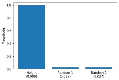
Based on the weight coefficients visualized above, we can see that “Height” is the feature that influences the prediction most. The two random features (Random 1 and Random 2) barely affect the model prediction. Since the prediction, based on the weights \(w_i\) and features \(x_i\), is defined as
\[\hat{y} = b + \sum_{i=1} w_ix_i\]we know that increasing the standardized height by 1 unit increases the prediction (standardized body weight) by 0.999 units (since \(w_{\text{height}}=0.999\)), i.e.,
\[\hat{y}_{x_\text{height} + 1} = \hat{y} +x_\text{height}w_{\text{height}} = \hat{y} +w_{\text{height}}.\]However, standardized features make it a bit more tricky to interpret the relationship between the original features and the target variable. To find out how much this increase of the target by 0.999 units means in terms of the non-standardized prediction (height in centimeters), we have to convert the z-score normalized target back onto the original scale. In other words, we have to undo the standardization formula
\[z'_{j} = \frac{z_j - \mu_j}{\sigma_j},\]that is,
\[z_{j} = z'_j \times \sigma_j + \mu_j.\]In the two equations above, \(z_j\) can denote the target variable (\(y\)), prediction (\(\hat{y}\)) or \(j\)-th feature (\(x_j\)) since the same concept applies.
Revisiting the example above, the model predicts \(\hat{y}=0.5\) (65.477kg) for a given input. We increase the standardized height by 1, which increases the prediction to approximately \(\hat{y}=1.5\) (72.276 kg). How much does this increase by 1 mean in terms of the target variable’s original scale \(y\)? We can compute this as follows:
\[(1.5\sigma_{\text{mass}}+\mu_{\text{mass}}) - (0.5\sigma_{\text{mass}}+\mu_{\text{mass}}) = \sigma_{\text{mass}}.\]Using the mean and variance stored in the StandardScaler instance we defined earlier, we can do this programmatically:
# y = 0.5 in kg
print(0.5 * np.sqrt(sc_target.var_) + sc_target.mean_)
# [65.4774427]

# y = 1.5 in kg
print(1.5 * np.sqrt(sc_target.var_) + sc_target.mean_)
# [72.2763281]

# sigma_mass:
print(np.sqrt(sc_target.var_))
# [6.7988854]
Next, after visualizing the model weights and exploring the relationship between a standardized and absolute feature and target values, we compute confidence intervals for the model weights. Using the equation defined earlier
\[\text{CI}_{1-\alpha}^{w_j} = \big[w_j - t_{\alpha / 2, n-2} \times SE(w_j), w_j + t_{\alpha / 2, n-2} \times SE(w_j) \big]\]with
\[S E\left(w_{i}\right)=\left(\frac{\sqrt{M S E}}{\sqrt{\sum_{i}\left(x_{j}^{(i)}-\bar{x}_{i}\right)^{2}}}\right)=\left(\frac{\sqrt{\frac{1}{n-2} \sum_{i}\left(y^{(i)}-y^{(i)}\right)^{2}}}{\sqrt{\sum_{i}\left(x_{j}^{(i)}-\bar{x}_{j}\right)^{2}}}\right),\]this amounts to
def std_err_linearregression(y_true, y_pred, x):
    n = len(y_true)
    mse = np.sum((y_true - y_pred)**2) / (n-2)
    std_err = (np.sqrt(mse) / np.sqrt(np.sum((x - np.mean(x, axis=0))**2, axis=0)))
    return std_err


def weight_intervals(n, weight, std_err, alpha=0.05):
    t_value = stats.t.ppf(1 - alpha/2, df=n - 2)
    temp = t_value * std_err
    lower = weight - temp
    upper = weight + temp

    return lower, upper


y_pred = lr.predict(X_std)
std_err = std_err_linearregression(y_std, y_pred, X_std)
lower, upper = weight_intervals(len(y_std), lr.coef_, std_err)
We can then visualize the weight cofficients and confidence intervals in an errorbar plot:
fig, ax = plt.subplots()

ax.hlines(0, xmin=-0.1, xmax=2.2, linestyle='dashed', color='skyblue')
ax.errorbar([0, 1, 2], lr.coef_, yerr=upper - lr.coef_, fmt='.k')

ax.set_xticks([0, 1, 2])
ax.set_xticklabels([f'Height\n({lr.coef_[0]:.3f})',
                    f'Random 1\n({lr.coef_[1]:.3f})',
                    f'Random 2\n({lr.coef_[2]:.3f})'])
plt.ylabel('Magnitude');
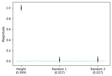
As we can see from the plot above, only the height feature is statstically significant at \(\alpha=0.05\).
If you are a Statsmodels user, an easier way to obtain the confidence intervals is as follows:
import statsmodels.api as sm


mod = sm.OLS(y_std, X_std)
res = mod.fit()
lower, upper = res.conf_int(0.05)[:, 0], res.conf_int(0.05)[:, 1]

########################
fig, ax = plt.subplots()

ax.hlines(0, xmin=-0.1, xmax=2.2, linestyle='dashed', color='skyblue')
ax.errorbar([0, 1, 2], res.params, yerr=upper - res.params, fmt='.k')

ax.set_xticks([0, 1, 2])
ax.set_xticklabels([f'Height\n({lr.coef_[0]:.3f})',
                    f'Random 1\n({lr.coef_[1]:.3f})',
                    f'Random 2\n({lr.coef_[2]:.3f})'])
plt.ylabel('Magnitude');
Logistic Regression
Logistic regression, being a generalized linear model (GLM), enjoys almost the same benefits as linear regression when interpreting model weights. (Of course, we use it for different purposes: logistic regression for predicting class labels and linear regression is for predicting continuous targets on a linear scale.)
Similar to linear regression, if we fit a logistic regression model to standardized features, we can look at the weights’ magnitudes to get an idea of how important the corresponding features are relative to each other. Generally, the larger the weight, the larger the impact of the corresponding feature on the prediction.
Both linear regression and logistic regression are GLMs, meaning that both use the weighted sum of features,
\[z = b + w_1x_1 + w_2x_2 + ...+ w_mx_m = b + \sum_j w_jx_j,\]to make predictions. In more technical terms, GLMs are models connecting the weighted sum, \(z\), to the mean of the target distribution using a link function. In the case of linear regression, the link function is simply an identity function. In logistic regression, the link function is a non-linear function (namely, the logistic sigmoid function). The logistic sigmoid function produces class membership probabilities for the target class (\(y=1\)) given features \(\mathbf{x}\):
\[P\left(y=1 | \mathbf{x}^{(i)}\right) = \frac{1}{1+ e ^{- z^{(i)} }}.\]Unfortunately, the link function makes interpreting the magnitudes of the weights slightly more complicated compared to linear regression. In linear regression, increasing a feature \(x_j\) by 1 adds \(w_j\) to the prediction (\(y\) becomes \(y+w_j\)). In logistic regression, changing \(x_j\) has a multiplicative rather than an additive effect on the prediction.
To see how changes in the input features affect the predictions, let us examine the relationship between predictions and the odds. The odds of an event (for instance, that a particular training example is classified as \(y=1\)) are written as the ratio between the probability of the event taking place and the probability of the event not taking place (this ratio is not to be confused with the so-called odds ratio):
\[\text{Odds}\left(\mathbf{x}^{(i)}\right) = \frac{P\left(y=1 | \mathbf{x}^{(i)}\right) }{1 - P\left(y=1| \mathbf{x}^{(i)}\right)}.\]The relationship between odds and the weighted sum of features is as follows: \(\text{Odds}\left(\mathbf{x}^{(i)}\right) = \frac{P\left(y=1 | \mathbf{x}^{(i)}\right) }{1 - P\left(y=1| \mathbf{x}^{(i)}\right)} = e^{z^{(i)}},\)
since
\[\begin{align}\frac{P\left(y=1 | \mathbf{x}^{(i)}\right) }{1 - P\left(y=1| \mathbf{x}^{(i)}\right)} &= \frac{\frac{1}{1+e^{-z}}}{1-\frac{1}{1+e^{-z}}}\\ &= \frac{\frac{e^z}{1+e^z}}{1-\frac{e^z}{1+e^z}}\\ &= \frac{e^z}{1+e^z - e^z}\\ &=e^z . \end{align}\]Now, changing a feature \(x_j\) by 1 will result in the following odds ratio:
\[\frac{\text{Odds}\left(x_j^{(i)} + 1\right)}{\text{Odds}\left(x_j^{(i)}\right)} = e^{w_j}.\]This is because
\[e^z = e^{b + w_1x_1 + w_2 x_2 + ... + w_m x_m} = e^{w_1x_1} \cdot e^{b+ w_2 x_2 + ... + w_m x_m},\]such that for \(x_{j+1} = x_j + 1\) we have \(x_{j+1} w_j = x_jw_j + w_j\), which gives us
\[\frac{\text{Odds}\left(x_j^{(i)} + 1\right)}{\text{Odds}\left(x_j^{(i)}\right)} = \frac{e^{w_j + (b + w_1x_1 + w_2 x_2 + ... + w_m x_m)}}{e^{b + w_1x_1 + w_2 x_2 + ... + w_m x_m}}= e^{w_j}.\]To summarize, increasing a feature \(x_j\) by 1 will scale the odds by a factor of \(e^{w_j}\).
Numeric Example
To illustrate the multiplicative effect on the logistic regression odds upon increasing a feature value, let us look at a numeric example. Assuming we start with an odds ratio of 2 for a particular example \(x^{(i)}\):
\[\text{Odds}\left(\mathbf{x}^{(i)}\right) = \frac{P\left(y=1 | \mathbf{x}^{(i)}\right) }{1 - P\left(y=1| \mathbf{x}^{(i)}\right)} = 2.\]We now increase the \(j\)-th feature by 1, that is, we increase the weighted sum by \(w_j\). Assuming \(w_j=1.1\), the odds ratio is then
\[\frac{\text{Odds}\left(x_j^{(i)} + 1\right)}{\text{Odds}\left(x_j^{(i)}\right)} = e^{w_j} = e^{1.1} = 3.\]This increases the odds in favor of assigning the class membership \(y=1\) by a factor 3 (from \(2\) to \(2 \cdot 3=6\)). In other words, the odds in favor of the event \(y=1\) increased 3-fold.
We can also look at this change in terms of the predicted class-membership probability
\[P\left(y=1 | \mathbf{x}^{(i)}\right).\]In logistic regression, the relationship between the predicted class-membership probability and the odds is as follows:
\[P\left(y=1 | \mathbf{x}^{(i)}\right) = \frac{1}{1 + e^{-z^{(i)}}} = \frac{e^{z^{(i)}}}{1 + e^{z^{(i)}}} = \frac{e^{\log\left(\text{Odds}\left(\mathbf{x}^{(i)}\right)\right)}}{1 + e^{\log(\text{Odds}\left(\left(\mathbf{x}^{(i)}\right)\right)}} = \frac{\text{Odds}\left(\mathbf{x}^{(i)}\right)}{1+\text{Odds}\left(\mathbf{x}^{(i)}\right)}.\]Starting with \(\text{Odds}\left(\mathbf{x}^{(i)}\right)=2\), the probability for \(\mathbf{x}^{(i)}\) being classified as \(y=1\) is \(2/(1+2) = 0.6667\).
Now, changing \(x_j\) by 1 unit, that is, scaling the odds ratio by \(e^{w_j}\) and assuming \(w_j=1.1\), updates the odds from 2 to \(2\cdot 3=6\). Consequently, plugging the odds into the equation above, the predicted class-membership probability,
\[P\left(y=1|\mathbf{x}^{(i)}\right),\]increases from \(2/3 = 0.6667\) to \(6/(1+6)=0.857\) .
Alternatively, we can also look at the impact of a feature increase from the perspective of the weighted inputs \(z = b + \sum_j w_j x_j\). For example, assume the weighted inputs, \(z = \log(2)=0.693\), then
\[\frac{1}{1 + e^{-\log(2)}}=2/3=0.6667.\]And increasing the the input by 1.1 gives us \(\frac{1}{1 + e^{- (\log(2)+1.1)}} = 0.857.\)
To summarize, increasing a feature \(x_j\) by 1 scales the odds ratio by \(e^{w_j}\), which means that the predicted class-membership probability changes from
\[\frac{\text{Odds}\left(\mathbf{x}^{(i)}\right)}{1+\text{Odds}\left(\mathbf{x}^{(i)}\right)}\]to
\[\frac{\text{Odds}\left(\mathbf{x}^{(i)}\right) \cdot e^{w_j}}{1+\text{Odds}\left(\mathbf{x}^{(i)}\right) \cdot e^{w_j}}.\]Confidence Intervals for Logistic Regression Weights
After the elaborate examples illustrating how changes in the feature values associated with logistic regression weights influence the prediction, let us briefly go over the general procedure for attaching confidence intervals to the model weights. Since this is already a long article, I will try to keep it short, and a thorough explanation can probably be found in most statistics textbooks.
In short, assuming that the model weights are asymptotically normal, we can compute the standard errors from the parameter covariance (or variance-covariance matrix) – the standard errors are the square root of the diagonal of the covariance matrix. We can then use these standard errors (similar to the previous linear regression example) to construct confidence intervals.
The covariance matrix can be written as
\[\Sigma = \mathbf{(X}^{T}\mathbf{V}\mathbf{X)}^{-1},\]where \(\mathbf{X}\) is the design matrix (\(m\) is the number of features, \(n\) is the number of training examples):
\[\mathbf{X = }\begin{bmatrix} 1 & x^{(1)}_{1} & \ldots & x^{(1)}_{p} \\ 1 & x^{(2)}_{1} & \ldots & x^{(2)}_{m} \\ \vdots & \vdots & \ddots & \vdots \\ 1 & x^{(n)}_{1} & \ldots & x^{(n)}_{m} \end{bmatrix};\]The column of 1’s is added for the model’s bias unit. \(\mathbf{V}\) is a diagonal matrix filled with each the variance of the predicted class membership probabilities,
\[p^{(i)} = P\left(y=1|\mathbf{x}^{(i)}\right):\] \[\mathbf{V = } \begin{bmatrix} \hat{p}^{(1)}(1 - \hat{p}^{(1)}) & 0 & \ldots & 0 \\ 0 & \hat{p}^{(2)}(1 - \hat{(p}^{(2)}) & \ldots & 0 \\ \vdots & \vdots & \ddots & \vdots \\ 0 & 0 & \ldots & \hat{p}^{(n)}(1 - \hat{p}^{(n)}) \end{bmatrix}.\]The standard errors (SE) are the square root of the diagonal of \(\Sigma\), and the confidence interval can be computed similar to linear regression as explained earlier:
\[\text{CI}_{1-\alpha}^{w_j} = \big[w_j - t_{\alpha / 2, n-2} \times SE(w_j), w_j + t_{\alpha / 2, n-2} \times SE(w_j) \big].\]Code Example
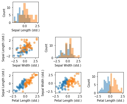
To make these concepts behind logistic regression more concrete, let us look at Python code examples. To focus on the method rather than the dataset, we will use a simplified version of the Iris dataset: 50 Versicolor flowers and 50 Virginia flowers. The features we consider are sepal length, sepal width, and petal width.
As it is common, we start with a simple visual sanity check using a scatterplot matrix after loading the dataset:
import matplotlib.pyplot as plt

from mlxtend.plotting import scatterplotmatrix
from sklearn.linear_model import LogisticRegression
from sklearn.preprocessing import StandardScaler
from sklearn.datasets import load_iris
from scipy import stats
import numpy as np


# Load and standardize dataset
iris = load_iris()

X_train, y_train = iris.data[50:150, :3], iris.target[50:150]
y_train = np.array(50*[0] + 50*[1])

sc_features = StandardScaler()
sc_target = StandardScaler()

X_std = sc_features.fit_transform(X_train)

# Plot dataset
fig, axes = scatterplotmatrix(X_std[y_train==0], figsize=(6, 5), alpha=0.5)
fig, axes = scatterplotmatrix(X_std[y_train==1], fig_axes=(fig, axes), alpha=0.5,
                              names=['Sepal Length (std.)','Sepal Width (std.)', 'Petal Length (std.)'])

plt.tight_layout()
plt.show()
Next, we are fitting a logistic regression model from scikit-learn on the standardized Iris features and plot the model weights:
lor = LogisticRegression(random_state=0, solver='newton-cg', C=1e8)

# set C=1e8 to negate regularization to allow comparison with
# statsmodel coefficients later

lor.fit(X_std, y_train)

fig, ax = plt.subplots()
ax.bar([0, 1, 2], lor.coef_.flatten())

ax.set_xticks([0, 1, 2])
ax.set_xticklabels([f'Sepal Length\n({lor.coef_.flatten()[0]:.3f})',
                    f'Sepal Width\n({lor.coef_.flatten()[1]:.3f})',
                    f'Petal Length\n({lor.coef_.flatten()[2]:.3f})'])
plt.ylabel('Magnitude')
plt.show()

As we can see in the barplot above, the petal length appears to be the dominant feature for distinguishing between Versicolor and Virginia flowers. This is consistent with our observations in the scatterplot matrix: looking at the petal length histogram in the lower right corner, it is intuitive to see that a linear classifier could separate the two species relatively well. The sepal width feature appears to be the least useful feature of a linear classifier, which is reflected in both the scatterplot matrix and the magnitude of the logistic regression model weights.
The standard errors can be computed from the covariance matrix, as explained in the previous section. The confidence intervals for the model weights can then be computed using the same procedure as for linear regression (the weight_interval code below is, in fact, identical to the previous weight_interval code and just included here for easier reference):
def std_err_logisticregression(y_true, y_pred_proba, X):
    # based on code from
    # https://stats.stackexchange.com/questions/89484/how-to-compute-the-standard-errors-of-a-logistic-regressions-coefficients

    # Design matrix -- add column of 1's at the beginning of your X_train matrix
    X_design = np.hstack([np.ones((X.shape[0], 1)), X])

    # Initiate matrix of 0's, fill diagonal with each predicted observation's variance
    V = np.diagflat(np.product(y_pred_proba, axis=1))

    # Covariance matrix
    cov = np.linalg.inv(X_design.T @ V @ X_design)

    # Standard errors:
    std_errs = np.sqrt(np.diag(cov))

    return std_errs


def weight_intervals(n, weight, std_err, alpha=0.05):
    t_value = stats.t.ppf(1 - alpha/2, df=n - 2)
    temp = t_value * std_err
    lower = weight - temp
    upper = weight + temp

    return lower, upper
y_pred_proba = lor.predict_proba(X_std)
std_err = std_err_logisticregression(y_train, y_pred_proba, X_std)

lower, upper = weight_intervals(len(y_train), lor.coef_.flatten(), std_err[1:])
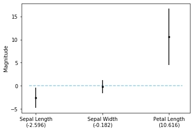
After computing the upper and lower confidence bounds (here, we are using a 95% confidence interval), we can visualize the interval in an errorbar plot:
fig, ax = plt.subplots()

ax.hlines(0, xmin=-0.1, xmax=2.2, linestyle='dashed', color='skyblue')
ax.errorbar([0, 1, 2], lor.coef_.flatten(), yerr=upper - lor.coef_.flatten(), fmt='.k')

ax.set_xticks([0, 1, 2])
ax.set_xticklabels([f'Sepal Length\n({lor.coef_.flatten()[0]:.3f})',
                    f'Sepal Width\n({lor.coef_.flatten()[1]:.3f})',
                    f'Petal Length\n({lor.coef_.flatten()[2]:.3f})'])
plt.ylabel('Magnitude');

As we can see from the plot above, both the sepal length and the petal length features are statistically significant.
Instead of computing the confidence intervals manually, as above, we can also use Statsmodels, which has this functionality already built in:
import statsmodels.api as sm


model = sm.Logit(y_train, X_std)
res = model.fit(method='ncg')
lower, upper = res.conf_int(0.05)[:, 0], res.conf_int(0.05)[:, 1]

fig, ax = plt.subplots()

ax.hlines(0, xmin=-0.1, xmax=2.2, linestyle='dashed', color='skyblue')
ax.errorbar([0, 1, 2], res.params, yerr=upper - res.params, fmt='.k')

ax.set_xticks([0, 1, 2])
ax.set_xticklabels([f'Sepal Length\n({res.params[0]:.3f})',
                    f'Sepal Width\n({res.params[1]:.3f})',
                    f'Petal Length\n({res.params[2]:.3f})'])
plt.ylabel('Magnitude');
Conclusion
There are many more aspects of generalized linear models that I did not cover in this article. But since linear regression and logistic regression are commonly used “tools” in applied data science and machine learning, I hope this brief rundown of interpreting model weights is useful to you. As a follow-up, I recommend reading the chapter on generalized linear models and generative additive models from the Interpretable Machine Learning book: https://christophm.github.io/interpretable-ml-book/extend-lm.html.
A future blog post may explore tree-based models as interpretable machine learning models.
PS: Jupyter Notebooks with the code examples from this article are available on GitHub at https://github.com/rasbt/interpretable-ml-article.
Read Next
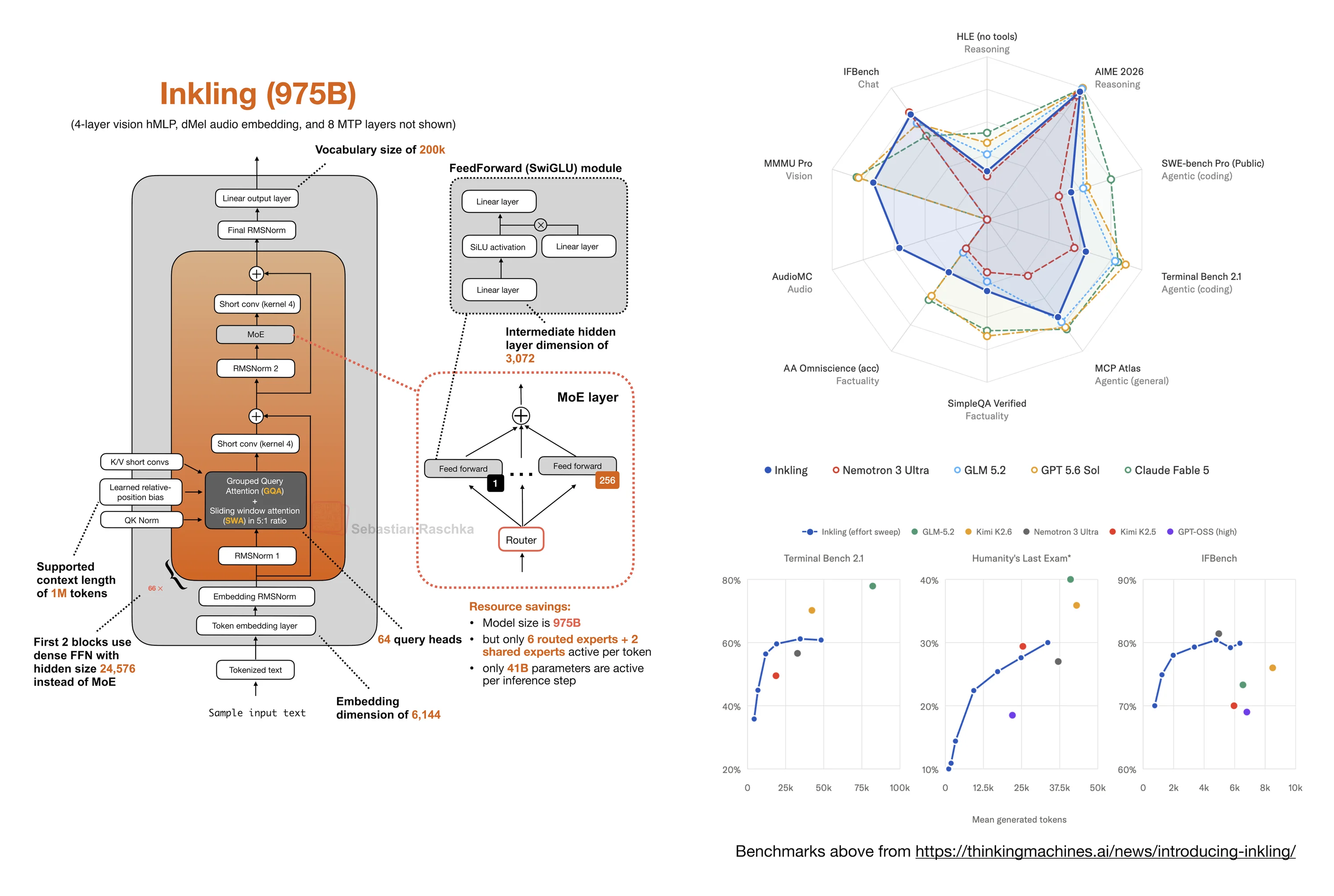 Inkling: A New Open-Weight 975B MoE with a Few Surprises
Short note on Thinking Machines Lab's 975B Inkling open-weight model, its benchmark profile, sparse MoE design, short convolutions, embedding RMSNorm, and
Inkling: A New Open-Weight 975B MoE with a Few Surprises
Short note on Thinking Machines Lab's 975B Inkling open-weight model, its benchmark profile, sparse MoE design, short convolutions, embedding RMSNorm, and
 200,000 Subscribers
Short note celebrating Ahead of AI reaching 200,000 subscribers.
200,000 Subscribers
Short note celebrating Ahead of AI reaching 200,000 subscribers.
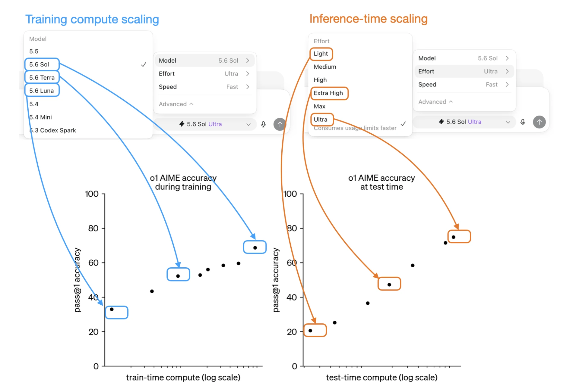 GPT 5.6 Has 72 Possible Configurations. What's A Good Default?
Short note on how GPT 5.6 model and effort choices map onto training-time and inference-time scaling, producing 72 configurations.
GPT 5.6 Has 72 Possible Configurations. What's A Good Default?
Short note on how GPT 5.6 model and effort choices map onto training-time and inference-time scaling, producing 72 configurations.

If you read the book and have a few minutes to spare, I'd really appreciate a brief review. It helps us authors a lot!
Your support means a great deal! Thank you!