My First Year at UW-Madison and a Gallery of Awesome Student Projects
Not too long ago, in the Summer of 2018, I was super excited to join the Department of Statistics at the University of Wisconsin-Madison after obtaining my Ph.D. after ~5 long and productive years. Now, two semesters later after finals’ week, I finally found some quiet days to look back on what’s happened since then.
During my first year at UW-Madison, besides moving my research projects forward, my life was centered around the two courses I was teaching (~70 students each!). In fall, I started with designing and teaching a new Machine Learning course, and after a relatively short 2-week winter break, I did the same with a new Deep Learning course this spring. Since these were new courses/topics in our department, I started from scratch concerning lecture material. I really like that, actually; however, it also was a lot of work! And in the end, it was very rewarding!
Both courses included various homework assignments as well as final exams. However, the fascinating parts were the individual class projects the students were working on. For these class projects, the ~70 students/class could choose their own topic, and it consisted of three stages:
- A project proposal; a short 3-page write-up (not quite as involved as a grant proposal ;)) to motivate and describe their project. This was an excellent opportunity for both the students and me to get/provide some guidance ~mid-semester before committing to the plan.
- A ~10-min presentation at the end of the semester to practice communication skills as well as sharing interesting results and valuable experiences with the other students – in the spirit of a small conference.
- A final ~8-page report modeled after a CVPR conference paper (mainly because it is a nice template) to practice written communication skills and gain practice concerning further research endeavors.
If you are interested and/or find it useful, all my lecture material is available on GitHub:
Below, I wanted to share some of the project the students were working on (we had 46 projects from both classes combined). Please note that I didn’t cherry-pick these projects below. I only selected those projects that students shared voluntarily – sharing their projects publicly was not a requirement in those courses.
(Please also keep in mind that these projects were done by undergraduate students who haven’t had any experience with machine learning and deep learning before.)
Audio Classification Using Convolutional Neural Networks
In this project, Poet Larsen, Reng Chiz Der, and Noah Haselow were exploring modern approaches for audio classification. In particular, Poet, Reng, and Noah used deep learning architectures that were originally developed for computer vision, namely convolutional neural networks (CNNs). The students implemented CNN architectures to capture temporal relationships in audio clips from spectrograms. They found that a Gated-CNN architecture was particularly helpful for mitigating vanishing gradient effects.
Without a doubt, audio classification has many important applications due to the abundance of audio-enabled devices and technologies such as Apple’s Siri voice assistant or Amazon’s Echo devices. However, more importantly, progress in audio classification can improve accessibility for hearing-impaired people.
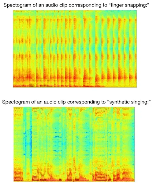
As a benchmark dataset for this study, the students used Google’s Voice Ontology AudioSet. The dataset was trimmed to 5000 audio clips and 10 classes due to computational processing constraints (the students observed that downloading all 2 million videos and convert them to audio clips would take approximately 3-5 months). After obtaining the 5000 clips, the students turned the audio samples into spectrograms via a discrete short-time Fourier transform. Two examples are shown below:
Primarily, the students focused on a Gated-CNN architecture, inspired by Dauphin and others (“Language modeling with gated convolutional networks”) and Xu and others (“Large-scale weakly supervised audio classification using gated convolutional neural network”):
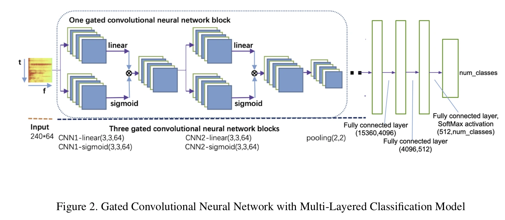
In this architecture, ReLU activations were replaced by learnable gated linear units (GLUs), which are somewhat similar to LSTMs or attention architectures, to help with vanishing gradient problems (also somewhat similar to ResNet architectures).
Furthermore, the students compared the Gated-CNN approach with other CNN architectures developed for image classification, such as VGG, AlexNet, and ResNet. The outcome is summarized in the two tables below:
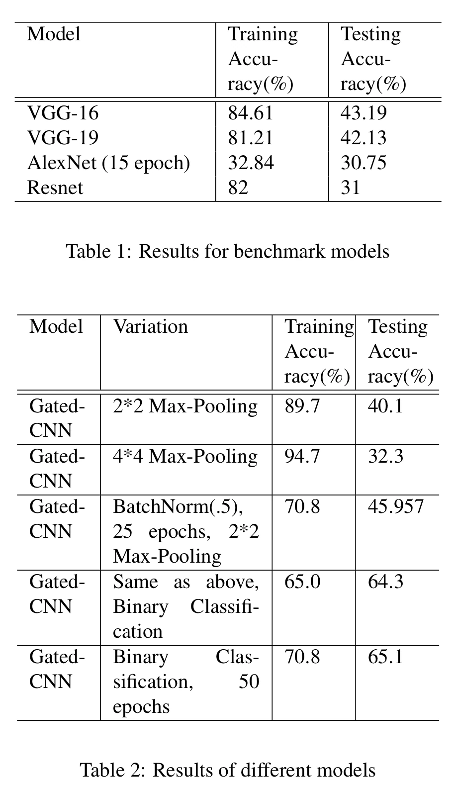
Looking at the training accuracy, the Gated-CNN models outperform the “conventional” image classification architectures for this audio classification from spectrograms. Interestingly, increasing the max-pooling size further improves the training accuracy. The students hypothesized that this might be because max-pooling helps to address the auto-correlation issue between neighboring sound slices. Unfortunately, all models suffer from a high degree of overfitting, though.
The overfitting issue may be due to the relatively small sample size (and a stronger dropout probability could potentially also help). Evidence for this is that In the bottom two rows, where the complexity of the classification task is reduced to a binary classification problem, the training-test gap was reduced substantially. It would be interesting to see how these architectures perform on the 10-class dataset with a larger number of training examples.
Despite the overfitting problems, all in all, this was an exciting project though that demonstrates that computer vision architectures can be useful for audio classification as well.
3D Convolutional Networks
In this project, the students took the opportunity to explore 3D-convolutional neural networks a bit further, since we only covered them briefly in the lecture. While traditional photographs are inarguably more wide-spread, there are many domains where 3D-data analysis is especially useful (in contrast to 3D movies). For instance, applications involving spatially aware self-driving cars and advanced medicine (i.e., medical imaging involving CT or MRI) are areas that benefit from deep learning technology that leverages the 3D-structure of the data.
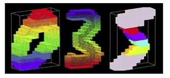
Since this study was performed for educational purposes, Sam Berglin, Jiahui Jian, and Lian Zheming used a 3D MNIST dataset to compare a “traditional” CNN architecture, an all-convolutional CNN architecture, and an architecture that the students refer to as “Connectome” – an architecture that was designed for fMRI data (traditionally, the term connectome refers to the wiring diagram of a biological nervous system). The 3D MNIST dataset consists of 3D point clouds generated from the original MNIST digits. Each 3D image contains 4096 pixels (16x16x16 pixels) and has 3 color channels obtained from voxelization (3x4096 = 12,288 pixels per image in total):
The dataset was then split into 10,000 training, 1,000 validation, and 1,000 test instances.
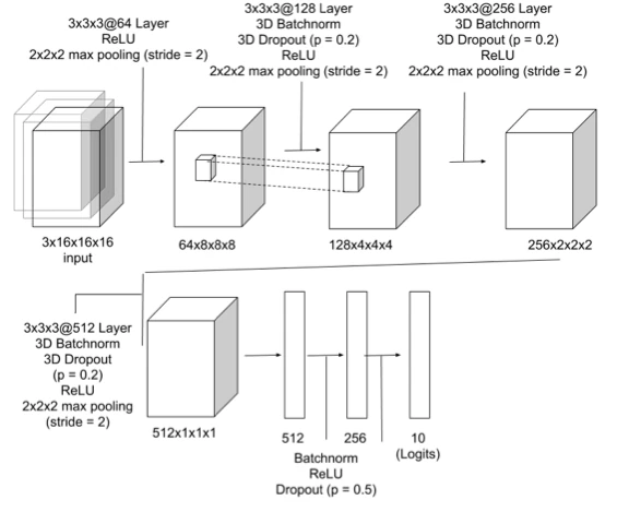
The students first implemented a relatively simple architecture with 3D convolutions, 3D dropout, 3D BatchNorm, and 3D max-pooling layers:
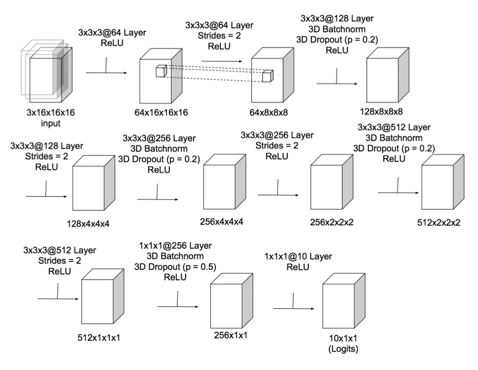
Then, inspired by Springenberg and other’s “All Convolutional Net,” the students replaced all max-pooling and fully connected layers by convolutional layers; however, the predictive performance remained essentially unchanged:
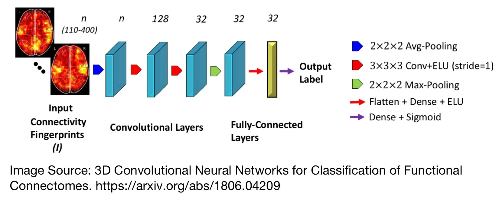
Next, the students implemented a so-called “Connectome” architecture as shown below:
While the “Connectome” architecture performed substantially worse than the traditional and all-convolutional CNN architectures, it shall be noted that it comes with the added benefit of a much smaller model size, which could make it particularly attractive for embedded devices:
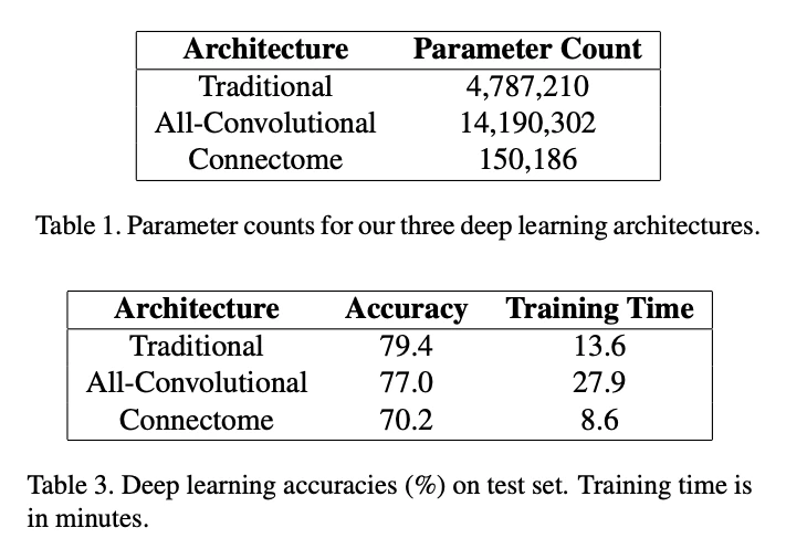
However, all CNN-based models compared very favorably to the baselines the students used in this study:
- Multinomial logistic regression: 52.6% test accuracy
- Random foresst: 52.1% test accuracy
- K-nearest neighbor: 55.3% test accuracy
As you may know, it’s relatively easy to achieve >90% test accuracy on the traditional 2D MNIST dataset with a generalized linear model such as multinomial logistic regression. Keeping that in mind, the performance of the CNN-based models is actually relatively good. Also, note that besides the challenge of having another dimension (16x more features), the number of training examples in the 3D MNIST dataset is also 5-times smaller compared to the original 2D MNIST dataset, which makes it easier to overfit.
Judging a Book by its Cover: A Modern Approach
Inspired by the common saying “do not judge a book by its cover,” the students were interested in finding out whether a “well-designed” book covers can indeed attract more readers – if this were true, this could obviously have useful real-world applications. To tackle this question, Yien Xu, Boyang Wei, and Jiongyi Cao composed the project of three subtasks:
- training a classification/ordinal regression CNN model to predict the popularity of a given book based on its cover image;
- using “model interpretation” algorithms to explain the predictions – which cover features contribute most towards predicting whether books are categorized as popular or unpopular;
- using a Generative Adversarial Nets (GAN) model to generate new popular book covers.
Note that the second point, interpreting the model, of course only makes sense if the classification/ordinal regression model can make reasonably good predictions. In the same spirit, if 1) and 2) result in satisfactory outcomes, this count as supporting evidence that the dataset contains sufficient information to model the popularity of books by their covers and that CNNs are able to extract this knowledge.
This project turned out to be the most creative project in this class (by the student voting consensus); at the same time, it was also the most ambitious one. While the generated book covers didn’t turn out to be very nice, it was an exciting project, nonetheless.
The dataset that the students used was Kaggle’s Goodreads’ Best Books Ever, which contained 53,618 book covers of various sizes (most of them are in RGB format). The labels were scores computed by Goodreads based on multiple factors, including user average ratings and review scores. The scores were given on a ranking scale, and to simplify the modeling problem, the students divided the ranking scale into five classes (from best to worst). Note that these class labels are on an ordinal (as opposed to a nominal scale). Hence, for the first subtask, predicting the popularity of book covers, the students used the CORAL framework for ordinal regression with CNNs that I recently developed with Wenzhi Cao and Vahid Mirjalili as opposed to a traditional Softmax+Cross-Entropy classifier approach.
The resulting training mean squared error (MAE) was 0.14, which is relatively reasonable given that a random prediction on a balanced dataset would result in an expected MAE of 2.5. However, the model, unfortunately, suffered from relatively severe overfitting as the test MAE as relatively high at 1.38. The students haven’t experimented with regularization techniques such as L2-norms or dropout, which could potentially help with alleviating this overfitting issue.
In any case, the students then proceeded with the model-interpretation part using Ribeiro and others’ LIME method. Personally, I would have recommended to leverage the fact that a CORAL-CNN is fully differentiable and used saliency maps or guided backpropagation, but LIME yielded some interesting insights, nonetheless, which can be seen in the Harry Potter example below (shown are the patches that contribute to books’ popularity the most):
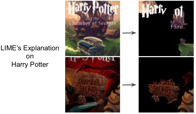
From the top row in the figure above, we can see that LIME correlated the book title itself with its popularity. In the bottom row, the students manually cropped the image to remove the title, and LIME then correlated the subtitle with the book’s popularity. In other words, we may hypothesize that the CNN model seemed to have learned to extract and base its predictions on the cover text rather than general image properties.
The third subtask, training a GAN for generating new book covers, was, unfortunately, a bit unsuccessful. However, it did produce some (almost) interesting book covers, as shown below:
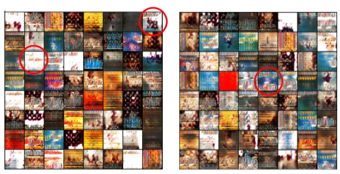
GANs are notoriously hard to train, and as we all know, it is common to do some cherry-picking when showing results. All in all, this was a very interesting project, and I really appreciated the focus on model interpretation!
Face-to-painting Machine
The analysis of face images is an increasingly popular area of research that gives rises to a large number of new algorithms and deep neural network architectures. The “Face-to-Painting Machine” by Lingfeng Zhu, Zhuoyan Xu, and Cecily Liu was centered around the exploration, comparison, and application of deep convolutional neural networks. The students’ main objective was the experimentation with face images, in particular, and they structured their project further into three subprojects:
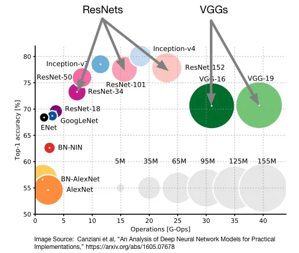
- comparing VGG and ResNet architectures for face recognition;
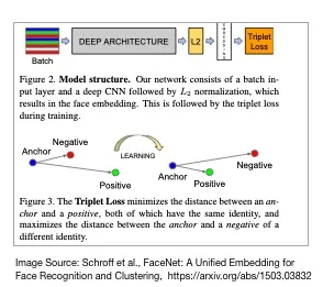
- performing face matching with triplet loss;
- using a deep-learning approach for photographic style transfer to apply various artistic styles to face images.
While the utility of face recognition in several important application areas, most prominently in the field of biometrics and security, the motivation behind neural style transfer may not be immediately apparent, the students gave an excellent explanation how it could fit into our modern world society:
Based on this feature and considering people’s crazy addiction to photograph editing apps, the applications of Neural Style Transfer could be extended to fancy filters for people to try out different filter effects. […] Besides, museums can use this method to repair damaged famous paintings or produce new ones.
Face Matching with Cross-Entropy Loss and Transfer Learning
For this part, the students built a custom web crawler to collect 7500 images from Google Image Search – the dataset contains images of 15 movie actors. The students then used pre-trained VGG and ResNet architectures for transfer learning and only trained the last, fully connected layers of each respective network for face matching. The resulting accuracy values are shown below (not that the photos are very diverse, and the expected accuracy of a random prediction is 6.7%):
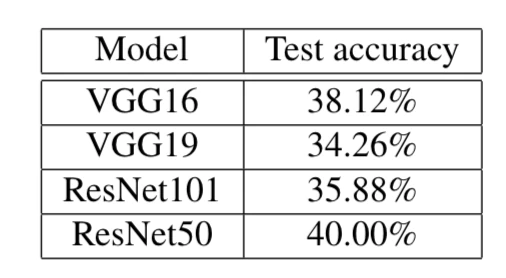
Note that due to computational limitations, the model was only trained for 10 hours (and did not fully converge). Other possible explanations for this relatively low performance are that the images are relatively diverse (they have not been cropped) and that the pre-trained models may not be ideal (if more data can be collected, training neural networks from scratch might yield better results.) In any case, the students then explored a more fruitful approach, i.e., using FaceNet’s triplet loss for learning face embeddings in a Euclidean space where distances directly correspond to facial similarity – a distance cutoff can then be used for face matching.
Face Matching with Triplet Loss
As shown below, the face matching performance using FaceNet’s triplet loss function improved was substantially improved:
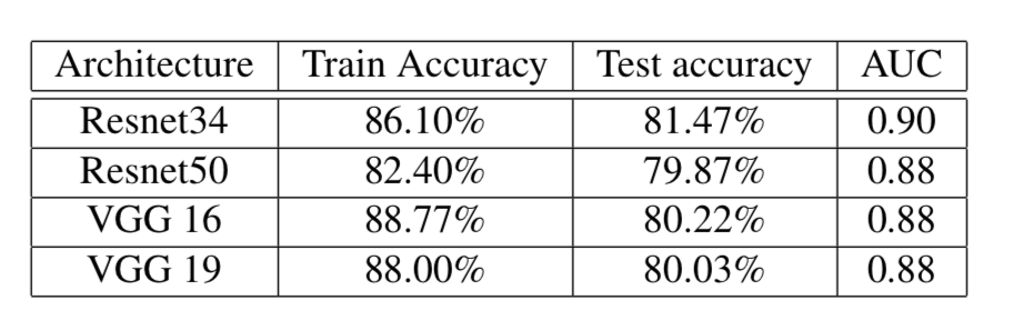
Interestingly, the smallest architecture (ResNet34) resulted in the best generalization performance. A potential explanation may be that the dataset was relatively small, and especially the VGG architectures may have suffered from an increasing degree of overfitting (increasing the dropout rate could potentially improve this situation).
For training the convolutional neural network models for face matching based on FaceNet’s triplet loss function, the students used the Labeled Face in the Wild (LFW) dataset. This dataset contained more than 13,000 face images collected from the internet, consisting of photographs of ~6000 different persons.
As suggested by the original FaceNet paper (Schroff and others, 2015), the students found that training on all positive-anchor and negative-anchor examples were not ideal (slow convergence).
Consequently, selecting only hard-negative and hard-positive examples in each minibatch for training may speed up the model fitting. However, even faster convergence (and more stable training) could be achieved when all anchor-positive examples were used. Now, by only selecting hard-negative examples, we can easily get trapped in local minima, because the gradients of the standard triplet loss are not symmetric, such that the negative-anchor pairs stop updating beyond a certain point as I illustrated below:
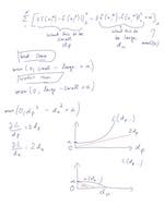
Hence, a better solution is to focus on the so-called “semi-hard” examples, which are anchor-negative pairs with a distance larger than the anchor-positive pairs but still “hard” since their measured distances are relatively close to the anchor-positive distances.
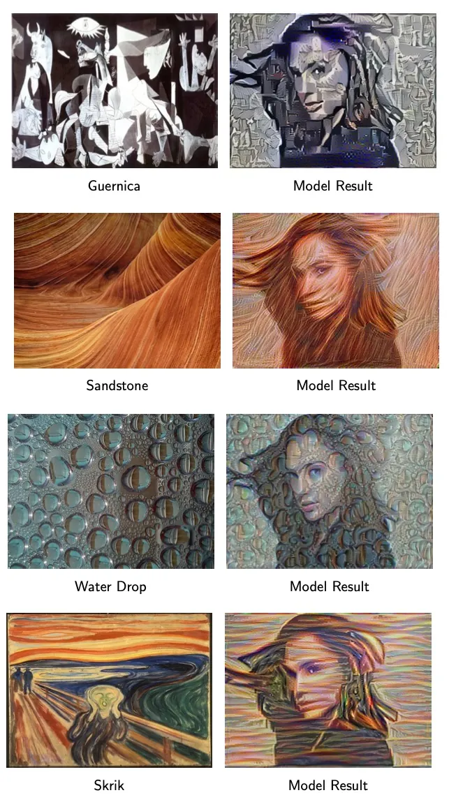
Photographic style transfer with deep learning
For this part, the students revisited their custom dataset consisting of 7500 images from Google Image Search – the dataset contains images of 15 movie actors. The style transfer approach, which the students outlined in more detail in their paper, yielded surprisingly nice results:
Music Genre Classification using Song Lyrics
Audio classification is undoubtly an interesting subject of study due to its large range of application areas: voice assistants like Apple’s Siri, Amazon’s Echo devices, to name a few. Also, from a privacy standpoint, there are many potentially interesting applications one could think of. For instance, music services such as Spotify heavily rely on user-based information for their recommendation engines. Especially, since we live in a day and age where personal information gets unintentionally leaked or intentionally sold, the exploration of alternative means for recommending “similar” songs might be of particular interest.
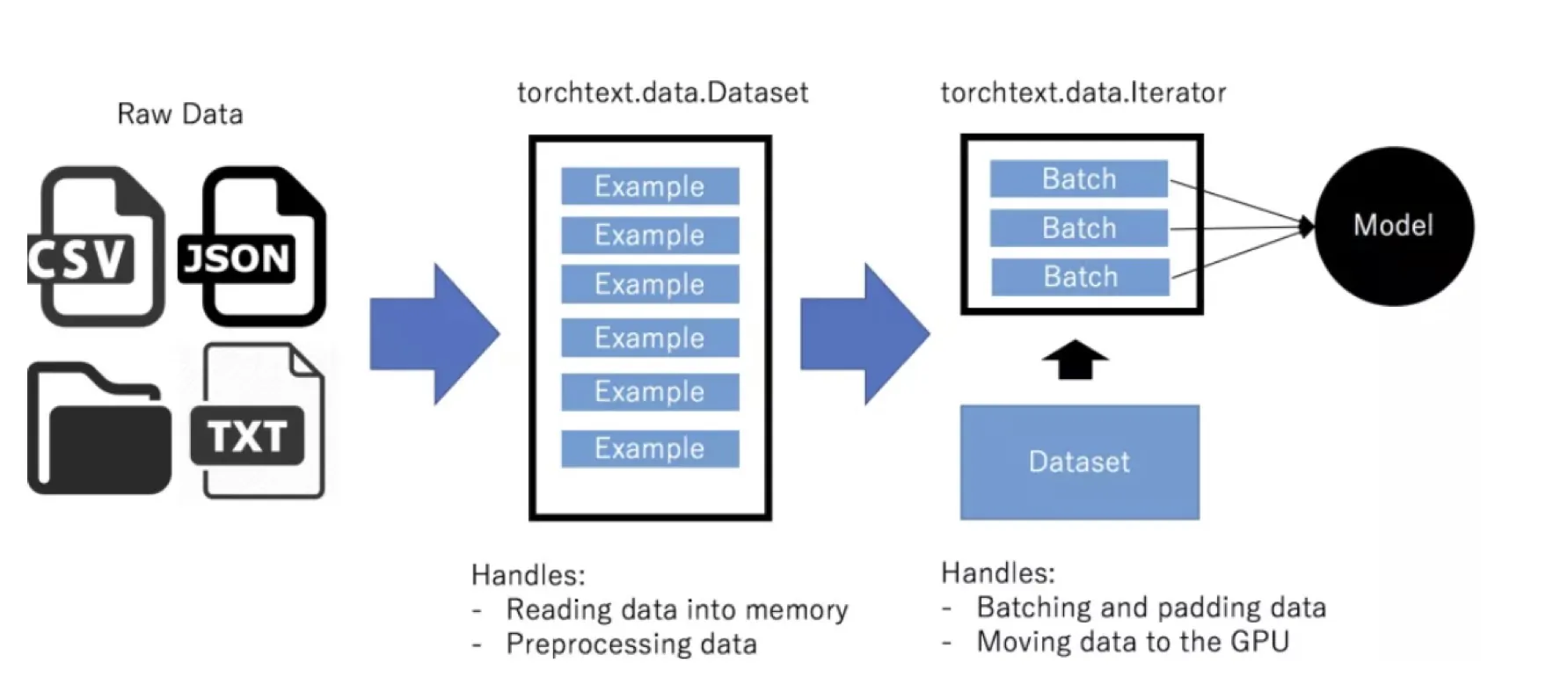
In this regard, Wengie Wang, Christina Gregis, and Yezhou Li explored whether song lyrics contain sufficient information to predict song genres. For this project, the students used the Million Song Dataset as a starting point and implemented several RNN architectures (a vanilla RNN, an RNN with Long Short-Term Memory, and an RNN with Gated Recurrent Units).
Unfortunately, the Million Song Dataset does not contain the lyrics itself; so, these had to be scraped from LyricWiki. The genre tags were obtained from Last.fm – note that these were user-based genre tags, which may not be the most accurate ones. While 1 million songs were used as a starting point, unfortunately, for only 1/5th of the songs both lyrics and genre tags were available (~220,000). And only about one-third of these 220,000 songs were associated with lyrics in English (for this project, it somewhat made sense not to mix multiple different languages).
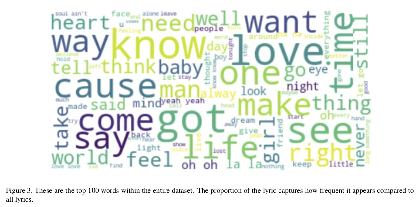
While ~70k may seem like a small dataset for training RNNs, the results looked (~70% test accuracy) quite good. However, as it turned out, the dataset was very imbalanced (towards rock songs), which led to an inflation of the accuracy score:
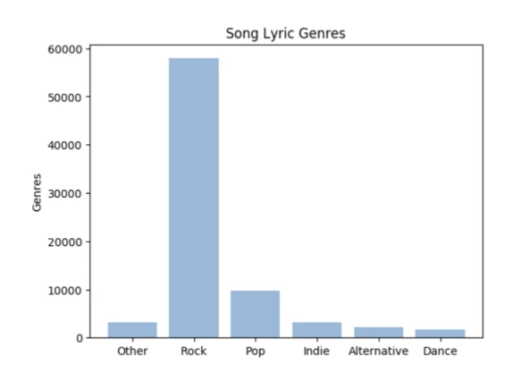
When the students balanced the dataset (only 9600 songs per genre), the predictive accuracy dropped substantially:
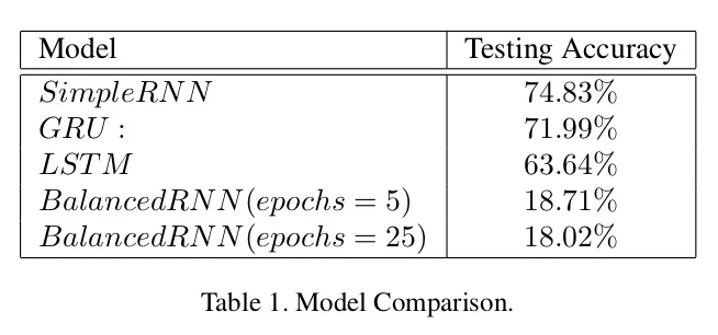
It seems that lyrics may not contain sufficient salient information to predict sing genres reliably. However, the low performance may also be due to the relatively small dataset size. It may be useful to explore “traditional” machine learning approaches, i.e., bag-of-words models with logistic regression or naive Bayes classifiers as a baseline. Also, another issue is that the user-assigned genre labels are relatively ambiguous, and genre boundaries are often also not very clear.
In any case, while the outcome, concerning predictive accuracy, was not a positive one, this was a nice and technically sound project, and a good educational exercise for implementing RNNs, which is not that trivial in PyTorch if you have a custom text dataset.
Projects from STAT479: Machine Learning
At last, below are two additional projects students shared from the “traditional machine learning” class I taught last semester, in Fall 2018.
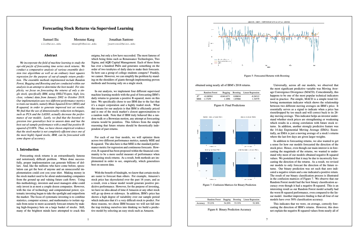
Forecasting Stock Returns via Supervised Learning
-
Authors: Samuel Ilic, Meenmo Kang, Jonathan Santoso
Abstract:
We incorporate the field of machine learning to study the age-old puzzle of forecasting time series stock returns. We conduct a comparative analysis of various ensemble deci- sion tree algorithms as well as an ordinary least squares regression for the purpose of out-of-sample return predic- tion. The ensemble methods implemented include Random Forest, Bagging and Boosting and are conducted within our analysis in an attempt to determine the best model. For sim- plicity, we focus on forecasting the returns of only a sin- gle stock, specifically IBM, using OHLCV(open, high, low, close, volume) data from January 2002 to October 2018. Our implementation uses two different performance metrics to train our models, namely Mean Squared Error (MSE) and R-squared, in order to generate improved test set results. We find that the use of dimensionality reduction techniques, such as PCA and the LASSO, actually decrease the perfor- mance of our models. Lastly, we find that the boosted re- gression tree generalizes best to unseen data and has the best out-of-sample performance with a small but positive R- squared of 0.06%. Thus, we have shown empirical evidence that the stock market is not completely efficient since one of the most highly liquid stocks, IBM, can be forecasted with some degree of accuracy.
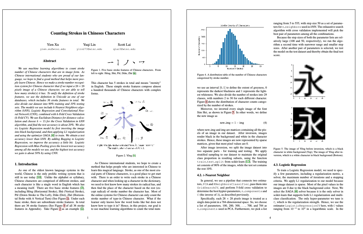
Counting Strokes in Chinese Characters
-
Authors: Yien Xu, Yuqi Lin, Scott Lai
Abstract:
We use machine learning algorithms to count stroke number of Chinese characters that are in image form. As Chinese international students who are proud of our lan- guage, we hope to find a good method that helps more peo- ple learn Chinese. Hence we make a stroke number recogni- tion system for Chinese character that if we input a 28 × 28 pixels image of a Chinese character, we are able to tell how many stroke(s) it has. To unify the definition of stroke features, we use the definition in Unicode as one of our databases, which includes 36 stroke features in total. We also divide our dataset into 90% training and 10% testing sets. The models we use include k-Nearest Neighbors algo- rithm (kNN), Logistic Regression and Convolutional Neu- ral Network (CNN), combined with k-Fold Cross Validation (k-Fold CV). We use Euclidean Distance for distance calcu- lation and choose k = 15 for the Cross Validation in kNN algorithm, and find the test accuracy is about 20%. We also try Logistic Regression model by first inverting the image into black background, and then applying L1 regularization and using the optimizer SAGA [4] to train. We obtain a test accuracy lower than kNN. By adding Bagging to Logistic Regression, we improve the accuracy a little bit. Logistic Regression with Max-Pooling gives the lowest test accuracy among all the models we use, and the highest test accuracy we gain is about 50% by using CNN.
Read Next
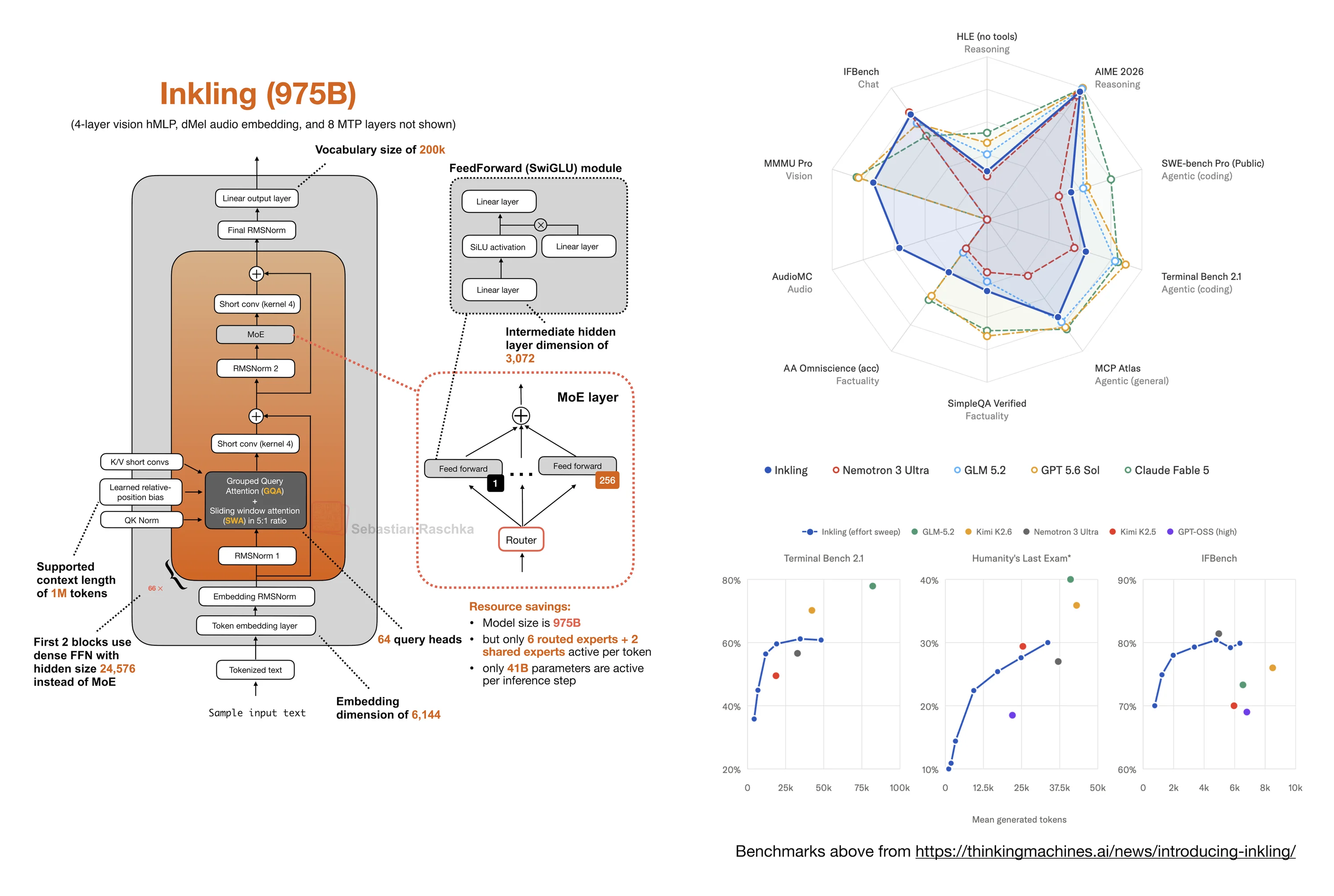 Inkling: A New Open-Weight 975B MoE with a Few Surprises
Short note on Thinking Machines Lab's 975B Inkling open-weight model, its benchmark profile, sparse MoE design, short convolutions, embedding RMSNorm, and
Inkling: A New Open-Weight 975B MoE with a Few Surprises
Short note on Thinking Machines Lab's 975B Inkling open-weight model, its benchmark profile, sparse MoE design, short convolutions, embedding RMSNorm, and
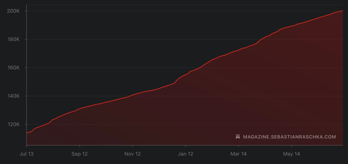 200,000 Subscribers
Short note celebrating Ahead of AI reaching 200,000 subscribers.
200,000 Subscribers
Short note celebrating Ahead of AI reaching 200,000 subscribers.
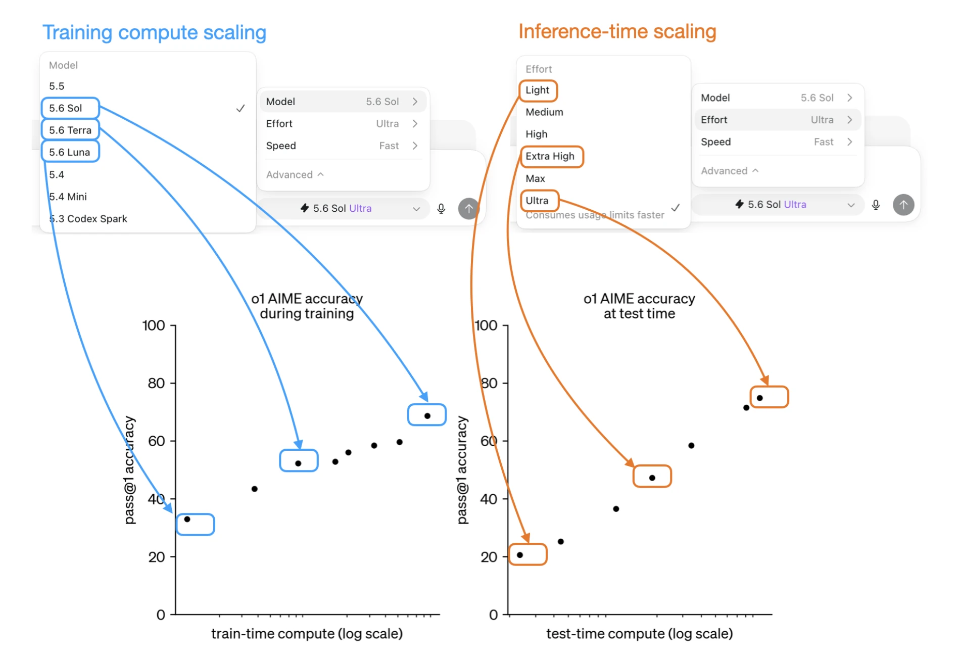 GPT 5.6 Has 72 Possible Configurations. What's A Good Default?
Short note on how GPT 5.6 model and effort choices map onto training-time and inference-time scaling, producing 72 configurations.
GPT 5.6 Has 72 Possible Configurations. What's A Good Default?
Short note on how GPT 5.6 model and effort choices map onto training-time and inference-time scaling, producing 72 configurations.

If you read the book and have a few minutes to spare, I'd really appreciate a brief review. It helps us authors a lot!
Your support means a great deal! Thank you!