An introduction to parallel programming using Python's multiprocessing module
– using Python's multiprocessing module
CPUs with multiple cores have become the standard in the recent development of modern computer architectures and we can not only find them in supercomputer facilities but also in our desktop machines at home, and our laptops; even Apple’s iPhone 5S got a 1.3 Ghz Dual-core processor in 2013.
However, the default Python interpreter was designed with simplicity in mind and has a thread-safe mechanism, the so-called “GIL” (Global Interpreter Lock). In order to prevent conflicts between threads, it executes only one statement at a time (so-called serial processing, or single-threading).
In this introduction to Python’s multiprocessing module, we will see how we can spawn multiple subprocesses to avoid some of the GIL’s disadvantages.
Sections
Multi-Threading vs. Multi-Processing
Depending on the application, two common approaches in parallel programming are either to run code via threads or multiple processes, respectively. If we submit “jobs” to different threads, those jobs can be pictured as “sub-tasks” of a single process and those threads will usually have access to the same memory areas (i.e., shared memory). This approach can easily lead to conflicts in case of improper synchronization, for example, if processes are writing to the same memory location at the same time.
A safer approach (although it comes with an additional overhead due to the communication overhead between separate processes) is to submit multiple processes to completely separate memory locations (i.e., distributed memory): Every process will run completely independent from each other.
Here, we will take a look at Python’s multiprocessing module and how we can use it to submit multiple processes that can run independently from each other in order to make best use of our CPU cores.
Introduction to the multiprocessing module
The multiprocessing module in Python’s Standard Library has a lot of powerful features. If you want to read about all the nitty-gritty tips, tricks, and details, I would recommend to use the official documentation as an entry point.
In the following sections, I want to provide a brief overview of different approaches to show how the multiprocessing module can be used for parallel programming.
The Process class
The most basic approach is probably to use the Process class from the multiprocessing module.
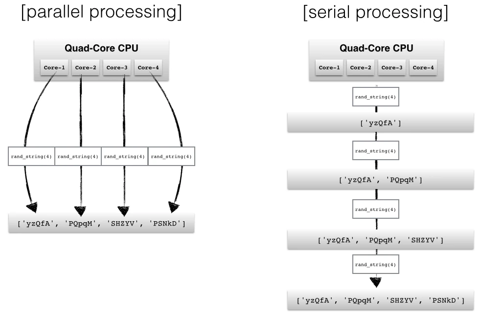
Here, we will use a simple queue function to generate four random strings in s parallel.
import multiprocessing as mp
import random
import string

random.seed(123)

# Define an output queue
output = mp.Queue()

# define a example function
def rand_string(length, output):
    """ Generates a random string of numbers, lower- and uppercase chars. """
    rand_str = ''.join(random.choice(
                        string.ascii_lowercase
                        + string.ascii_uppercase
                        + string.digits)
                   for i in range(length))
    output.put(rand_str)

# Setup a list of processes that we want to run
processes = [mp.Process(target=rand_string, args=(5, output)) for x in range(4)]

# Run processes
for p in processes:
    p.start()

# Exit the completed processes
for p in processes:
    p.join()

# Get process results from the output queue
results = [output.get() for p in processes]

print(results)
['BJWNs', 'GOK0H', '7CTRJ', 'THDF3']
How to retrieve results in a particular order
The order of the obtained results does not necessarily have to match the order of the processes (in the processes list). Since we eventually use the .get() method to retrieve the results from the Queue sequentially, the order in which the processes finished determines the order of our results.
E.g., if the second process has finished just before the first process, the order of the strings in the results list could have also been
['PQpqM', 'yzQfA', 'SHZYV', 'PSNkD'] instead of ['yzQfA', 'PQpqM', 'SHZYV', 'PSNkD']
If our application required us to retrieve results in a particular order, one possibility would be to refer to the processes’ ._identity attribute. In this case, we could also simply use the values from our range object as position argument. The modified code would be:
# Define an output queue
output = mp.Queue()

# define a example function
def rand_string(length, pos, output):
    """ Generates a random string of numbers, lower- and uppercase chars. """
    rand_str = ''.join(random.choice(
                        string.ascii_lowercase
                        + string.ascii_uppercase
                        + string.digits)
                   for i in range(length))
    output.put((pos, rand_str))

# Setup a list of processes that we want to run
processes = [mp.Process(target=rand_string, args=(5, x, output)) for x in range(4)]

# Run processes
for p in processes:
    p.start()

# Exit the completed processes
for p in processes:
    p.join()

# Get process results from the output queue
results = [output.get() for p in processes]

print(results)
[(0, 'h5hoV'), (1, 'fvdmN'), (2, 'rxGX4'), (3, '8hDJj')]
And the retrieved results would be tuples, for example, [(0, 'KAQo6'), (1, '5lUya'), (2, 'nj6Q0'), (3, 'QQvLr')]
or [(1, '5lUya'), (3, 'QQvLr'), (0, 'KAQo6'), (2, 'nj6Q0')]
To make sure that we retrieved the results in order, we could simply sort the results and optionally get rid of the position argument:
results.sort()
results = [r[1] for r in results]
print(results)
['h5hoV', 'fvdmN', 'rxGX4', '8hDJj']
A simpler way to maintain an ordered list of results is to use the Pool.apply and Pool.map functions which we will discuss in the next section.
The Pool class
Another and more convenient approach for simple parallel processing tasks is provided by the Pool class.
There are four methods that are particularly interesting:
-
Pool.apply -
Pool.map -
Pool.apply_async -
Pool.map_async
The Pool.apply and Pool.map methods are basically equivalents to Python’s in-built apply and map functions.
Before we come to the async variants of the Pool methods, let us take a look at a simple example using Pool.apply and Pool.map. Here, we will set the number of processes to 4, which means that the Pool class will only allow 4 processes running at the same time.
def cube(x):
    return x**3
pool = mp.Pool(processes=4)
results = [pool.apply(cube, args=(x,)) for x in range(1,7)]
print(results)
[1, 8, 27, 64, 125, 216]
pool = mp.Pool(processes=4)
results = pool.map(cube, range(1,7))
print(results)
[1, 8, 27, 64, 125, 216]
The Pool.map and Pool.apply will lock the main program until all processes are finished, which is quite useful if we want to obtain results in a particular order for certain applications.
In contrast, the async variants will submit all processes at once and retrieve the results as soon as they are finished.
One more difference is that we need to use the get method after the apply_async() call in order to obtain the return values of the finished processes.
pool = mp.Pool(processes=4)
results = [pool.apply_async(cube, args=(x,)) for x in range(1,7)]
output = [p.get() for p in results]
print(output)
[1, 8, 27, 64, 125, 216]
Kernel density estimation as benchmarking function
In the following approach, I want to do a simple comparison of a serial vs. multiprocessing approach where I will use a slightly more complex function than the cube example, which he have been using above.
Here, I define a function for performing a Kernel density estimation for probability density functions using the Parzen-window technique.
I don’t want to go into much detail about the theory of this technique, since we are mostly interested to see how multiprocessing can be used for performance improvements, but you are welcome to read my more detailed article about the Parzen-window method here.
import numpy as np

def parzen_estimation(x_samples, point_x, h):
    """
    Implementation of a hypercube kernel for Parzen-window estimation.

    Keyword arguments:
        x_sample:training sample, 'd x 1'-dimensional numpy array
        x: point x for density estimation, 'd x 1'-dimensional numpy array
        h: window width

    Returns the predicted pdf as float.

    """
    k_n = 0
    for row in x_samples:
        x_i = (point_x - row[:,np.newaxis]) / (h)
        for row in x_i:
            if np.abs(row) > (1/2):
                break
        else: # "completion-else"*
            k_n += 1
    return (k_n / len(x_samples)) / (h**point_x.shape[1])
A quick note about the “completion else
Sometimes I receive comments about whether I used this for-else combination intentionally or if it happened by mistake. That is a legitimate question, since this “completion-else” is rarely used (that’s what I call it, I am not aware if there is an “official” name for this, if so, please let me know).
I have a more detailed explanation here in one of my blog-posts, but in a nutshell: In contrast to a conditional else (in combination with if-statements), the “completion else” is only executed if the preceding code block (here the for-loop) has finished.
The Parzen-window method in a nutshell
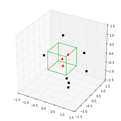
So what this function does in a nutshell: It counts points in a defined region (the so-called window), and divides the number of those points inside by the number of total points to estimate the probability of a single point being in a certain region.
Below is a simple example where our window is represented by a hypercube centered at the origin, and we want to get an estimate of the probability for a point being in the center of the plot based on the hypercube.
from mpl_toolkits.mplot3d import Axes3D
import matplotlib.pyplot as plt
import numpy as np
from itertools import product, combinations
fig = plt.figure(figsize=(7,7))
ax = fig.gca(projection='3d')
ax.set_aspect("equal")

# Plot Points

# samples within the cube
X_inside = np.array([[0,0,0],[0.2,0.2,0.2],[0.1, -0.1, -0.3]])

X_outside = np.array([[-1.2,0.3,-0.3],[0.8,-0.82,-0.9],[1, 0.6, -0.7],
                      [0.8,0.7,0.2],[0.7,-0.8,-0.45],[-0.3, 0.6, 0.9],
                      [0.7,-0.6,-0.8]])

for row in X_inside:
    ax.scatter(row[0], row[1], row[2], color="r", s=50, marker='^')

for row in X_outside:
    ax.scatter(row[0], row[1], row[2], color="k", s=50)

# Plot Cube
h = [-0.5, 0.5]
for s, e in combinations(np.array(list(product(h,h,h))), 2):
    if np.sum(np.abs(s-e)) == h[1]-h[0]:
        ax.plot3D(*zip(s,e), color="g")

ax.set_xlim(-1.5, 1.5)
ax.set_ylim(-1.5, 1.5)
ax.set_zlim(-1.5, 1.5)

plt.show()
point_x = np.array([[0],[0],[0]])
X_all = np.vstack((X_inside,X_outside))

print('p(x) =', parzen_estimation(X_all, point_x, h=1))
p(x) = 0.3
Sample data and timeit benchmarks
In the section below, we will create a random dataset from a bivariate Gaussian distribution with a mean vector centered at the origin and a identity matrix as covariance matrix.
import numpy as np

np.random.seed(123)

# Generate random 2D-patterns
mu_vec = np.array([0,0])
cov_mat = np.array([[1,0],[0,1]])
x_2Dgauss = np.random.multivariate_normal(mu_vec, cov_mat, 10000)
The expected probability of a point at the center of the distribution is ~ 0.15915 as we can see below.
And our goal is here to use the Parzen-window approach to predict this density based on the sample data set that we have created above.
In order to make a “good” prediction via the Parzen-window technique, it is - among other things - crucial to select an appropriate window with. Here, we will use multiple processes to predict the density at the center of the bivariate Gaussian distribution using different window widths.
from scipy.stats import multivariate_normal
var = multivariate_normal(mean=[0,0], cov=[[1,0],[0,1]])
print('actual probability density:', var.pdf([0,0]))
actual probability density: 0.159154943092
Benchmarking functions
Below, we will set up benchmarking functions for our serial and multiprocessing approach that we can pass to our timeit benchmark function.
We will be using the Pool.apply_async function to take advantage of firing up processes simultaneously: Here, we don’t care about the order in which the results for the different window widths are computed, we just need to associate each result with the input window width.
Thus we add a little tweak to our Parzen-density-estimation function by returning a tuple of 2 values: window width and the estimated density, which will allow us to sort our list of results later.
def parzen_estimation(x_samples, point_x, h):
    k_n = 0
    for row in x_samples:
        x_i = (point_x - row[:,np.newaxis]) / (h)
        for row in x_i:
            if np.abs(row) > (1/2):
                break
        else: # "completion-else"*
            k_n += 1
    return (h, (k_n / len(x_samples)) / (h**point_x.shape[1]))
def serial(samples, x, widths):
    return [parzen_estimation(samples, x, w) for w in widths]

def multiprocess(processes, samples, x, widths):
    pool = mp.Pool(processes=processes)
    results = [pool.apply_async(parzen_estimation, args=(samples, x, w)) for w in widths]
    results = [p.get() for p in results]
    results.sort() # to sort the results by input window width
    return results
Just to get an idea what the results would look like (i.e., the predicted densities for different window widths):
widths = np.arange(0.1, 1.3, 0.1)
point_x = np.array([[0],[0]])
results = []

results = multiprocess(4, x_2Dgauss, point_x, widths)

for r in results:
    print('h = %s, p(x) = %s' %(r[0], r[1]))
h = 0.1, p(x) = 0.016
h = 0.2, p(x) = 0.0305
h = 0.3, p(x) = 0.045
h = 0.4, p(x) = 0.06175
h = 0.5, p(x) = 0.078
h = 0.6, p(x) = 0.0911666666667
h = 0.7, p(x) = 0.106
h = 0.8, p(x) = 0.117375
h = 0.9, p(x) = 0.132666666667
h = 1.0, p(x) = 0.1445
h = 1.1, p(x) = 0.157090909091
h = 1.2, p(x) = 0.1685
Based on the results, we can say that the best window-width would be h=1.1, since the estimated result is close to the actual result ~0.15915.
Thus, for the benchmark, let us create 100 evenly spaced window width in the range of 1.0 to 1.2.
widths = np.linspace(1.0, 1.2, 100)
import timeit

mu_vec = np.array([0,0])
cov_mat = np.array([[1,0],[0,1]])
n = 10000

x_2Dgauss = np.random.multivariate_normal(mu_vec, cov_mat, n)

benchmarks = []

benchmarks.append(timeit.Timer('serial(x_2Dgauss, point_x, widths)',
            'from __main__ import serial, x_2Dgauss, point_x, widths').timeit(number=1))

benchmarks.append(timeit.Timer('multiprocess(2, x_2Dgauss, point_x, widths)',
            'from __main__ import multiprocess, x_2Dgauss, point_x, widths').timeit(number=1))

benchmarks.append(timeit.Timer('multiprocess(3, x_2Dgauss, point_x, widths)',
            'from __main__ import multiprocess, x_2Dgauss, point_x, widths').timeit(number=1))

benchmarks.append(timeit.Timer('multiprocess(4, x_2Dgauss, point_x, widths)',
            'from __main__ import multiprocess, x_2Dgauss, point_x, widths').timeit(number=1))

benchmarks.append(timeit.Timer('multiprocess(6, x_2Dgauss, point_x, widths)',
            'from __main__ import multiprocess, x_2Dgauss, point_x, widths').timeit(number=1))
Preparing the plotting of the results
import platform

def print_sysinfo():

    print('\nPython version  :', platform.python_version())
    print('compiler        :', platform.python_compiler())

    print('\nsystem     :', platform.system())
    print('release    :', platform.release())
    print('machine    :', platform.machine())
    print('processor  :', platform.processor())
    print('CPU count  :', mp.cpu_count())
    print('interpreter:', platform.architecture()[0])
    print('\n\n')
from matplotlib import pyplot as plt
import numpy as np

def plot_results():
    bar_labels = ['serial', '2', '3', '4', '6']

    fig = plt.figure(figsize=(10,8))

    # plot bars
    y_pos = np.arange(len(benchmarks))
    plt.yticks(y_pos, bar_labels, fontsize=16)
    bars = plt.barh(y_pos, benchmarks,
             align='center', alpha=0.4, color='g')

    # annotation and labels

    for ba,be in zip(bars, benchmarks):
        plt.text(ba.get_width() + 2, ba.get_y() + ba.get_height()/2,
                '{0:.2%}'.format(benchmarks[0]/be),
                ha='center', va='bottom', fontsize=12)

    plt.xlabel('time in seconds for n=%s' %n, fontsize=14)
    plt.ylabel('number of processes', fontsize=14)
    t = plt.title('Serial vs. Multiprocessing via Parzen-window estimation', fontsize=18)
    plt.ylim([-1,len(benchmarks)+0.5])
    plt.xlim([0,max(benchmarks)*1.1])
    plt.vlines(benchmarks[0], -1, len(benchmarks)+0.5, linestyles='dashed')
    plt.grid()

    plt.show()
Results
plot_results()
print_sysinfo()
Python version  : 3.4.1
compiler        : GCC 4.2.1 (Apple Inc. build 5577)

system     : Darwin
release    : 13.2.0
machine    : x86_64
processor  : i386
CPU count  : 4
interpreter: 64bit
Conclusion
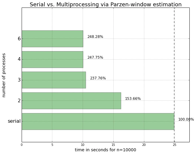
We can see that we could speed up the density estimations for our Parzen-window function if we submitted them in parallel. However, on my particular machine, the submission of 6 parallel 6 processes doesn’t lead to a further performance improvement, which makes sense for a 4-core CPU.
We also notice that there was a significant performance increase when we were using 3 instead of only 2 processes in parallel. However, the performance increase was less significant when we moved up to 4 parallel processes, respectively.
This can be attributed to the fact that in this case, the CPU consists of only 4 cores, and system processes, such as the operating system, are also running in the background. Thus, the fourth core simply does not have enough capacity left to further increase the performance of the fourth process to a large extend. And we also have to keep in mind that every additional process comes with an additional overhead for inter-process communication.
Also, an improvement due to parallel processing only makes sense if our tasks are “CPU-bound” where the majority of the task is spent in the CPU in contrast to I/O bound tasks, i.e., tasks that are processing data from a disk.
Read Next
 Scientific Computing in Python: Introduction to NumPy and Matplotlib
Beginner's guide to NumPy and Matplotlib for scientific computing: arrays, indexing, broadcasting, linear algebra, and plotting with Python code examples.
Scientific Computing in Python: Introduction to NumPy and Matplotlib
Beginner's guide to NumPy and Matplotlib for scientific computing: arrays, indexing, broadcasting, linear algebra, and plotting with Python code examples.
 Model evaluation, model selection, and algorithm selection in machine learning
Part 4 of the model evaluation series explaining statistical tests, algorithm comparisons, corrected resampled tests, and nested cross-validation.
Model evaluation, model selection, and algorithm selection in machine learning
Part 4 of the model evaluation series explaining statistical tests, algorithm comparisons, corrected resampled tests, and nested cross-validation.
 Generating Gender-Neutral Face Images with Semi-Adversarial Neural Networks to Enhance Privacy
I thought that it would be nice to have short and concise summaries of recent projects handy, to share them with a more general audience, including...
Generating Gender-Neutral Face Images with Semi-Adversarial Neural Networks to Enhance Privacy
I thought that it would be nice to have short and concise summaries of recent projects handy, to share them with a more general audience, including...

If you read the book and have a few minutes to spare, I'd really appreciate a brief review. It helps us authors a lot!
Your support means a great deal! Thank you!