At its core, this article is about a simple cheat sheet for basic operations on numeric matrices, which can be very useful if you working and experimenting with some of the most popular languages that are used for scientific computing, statistics, and data analysis.

Sections

• Sections
• Introduction
  • Language overview
• MATLAB/Octave
  • GNU Octave
• Python NumPy
• R
• Julia
• Cheat sheet
  • Alternative data structures: NumPy matrices vs. NumPy arrays

Introduction

Matrices (or multidimensional arrays) are not only presenting the fundamental elements of many algebraic equations that are used in many popular fields, such as pattern classification, machine learning, data mining, and math and engineering in general. But in context of scientific computing, they also come in very handy for managing and storing data in an more organized tabular form.
Such multidimensional data structures are also very powerful performance-wise thanks to the concept of automatic vectorization: instead of the individual and sequential processing of operations on scalars in loop-structures, the whole computation can be parallelized in order to make optimal use of modern computer architectures.

Language overview

Before we jump to the actual cheat sheet, I wanted to give you at least a brief overview of the different languages that we are dealing with.

All four languages, MATLAB/Octave, Python, R, and Julia are dynamically typed, have a command line interface for the interpreter, and come with great number of additional and useful libraries to support scientific and technical computing. Conveniently, these languages also offer great solutions for easy plotting and visualizations.

Combined with interactive notebook interfaces or dynamic report generation engines (MuPAD for MATLAB, IPython Notebook for Python, knitr for R, and IJulia for Julia based on IPython Notebook) data analysis and documentation has never been easier.

MATLAB/Octave

MATLAB (stands for MATrix LABoratory) is the name of an application and language that was developed by MathWorks back in

1. One of its strengths is the variety of different and highly optimized “toolboxes” (including very powerful functions for image and other signal processing task), which makes suitable for tackling basically every possible science and engineering task.
   Like the other languages, which will be covered in this article, it has cross-platform support and is using dynamic types, which allows for a convenient interface, but can also be quite “memory hungry” for computations on large data sets.

Even today, MATLAB is probably (still) the most popular language for numeric computation used for engineering tasks in academia as well as in industry.

GNU Octave

It is also worth mentioning that MATLAB is the only language in this cheat sheet which is not free and open-sourced. But since it is so immensely popular, I want to mention it nonetheless. And as an alternative there is also the free GNU Octave re-implementation that follows the same syntactic rules so that the code is compatible to MATLAB (except for very specialized libraries).

This image is a freely usable media under public domain and represents the first eigenfunction of the L-shaped membrane, resembling (but not identical to) MATLAB’s logo trademarked by MathWorks Inc.

Python NumPy

Initially, the NumPy project started out under the name “Numeric” in 1995 (renamed to NumPy in 2006) as a Python library for numeric computations based on multi-dimensional data structures, such as arrays and matrices. Since it makes use of pre-compiled C code for operations on its “ndarray” objects, it is considerably faster than using equivalent approaches in (C)Python.

Python NumPy is my personal favorite since I am a big fan of the Python programming language. Although similar tools exist for other languages, I found myself to be most productive doing my research and data analyses in IPython notebooks.
It allows me to easily combine Python code (sometimes optimized by compiling it via the Cython C-Extension or the just-in-time (JIT) Numba compiler if speed is a concern) with different libraries from the Scipy stack including matplotlib for inline data visualization (you can find some of my example benchmarks in this GitHub repository).

R

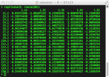
The R programming language was developed in 1993 and is a modern GNU implementation of an older statistical programming language called S, which was developed in the Bell Laboratories in 1976. Since its release, it has a fast-growing user base and is particularly popular among statisticians.

R was also the first language which kindled my fascination for statistics and computing. I have used it quite extensively a couple of years ago before I discovered Python as my new favorite language for data analysis.
Although R has great in-built functions for performing all sorts statistics, as well as a plethora of freely available libraries developed by the large R community, I often hear people complaining about its rather unintuitive syntax.

Julia

With its first release in 2012, Julia is by far the youngest of the programming languages mentioned in this article. a While Julia can also be used as an interpreted language with dynamic types from the command line, it aims for high-performance in scientific computing that is superior to the other dynamic programming languages for technical computing thanks to its LLVM-based just-in-time (JIT) compiler.

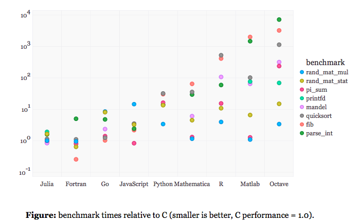
Personally, I haven’t used Julia that extensively, yet, but there are some exciting benchmarks that look very promising:

C compiled by gcc 4.8.1, taking best timing from all optimization levels (-O0 through -O3). C, Fortran and Julia use OpenBLAS v0.2.8. The Python implementations of rand_mat_stat and rand_mat_mul use NumPy (v1.6.1) functions; the rest are pure Python implementations.

Bezanson, J., Karpinski, S., Shah, V.B. and Edelman, A. (2012), “Julia: A fast dynamic language for technical computing”.
(Source: http://julialang.org/benchmarks/, with permission from the copyright holder)

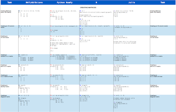
Cheat sheet

Alternative data structures: NumPy matrices vs. NumPy arrays

Python’s NumPy library also has a dedicated “matrix” type with a syntax that is a little bit closer to the MATLAB matrix: For example, the “ * ” operator would perform a matrix-matrix multiplication of NumPy matrices - same operator performs element-wise multiplication on NumPy arrays.

Vice versa, the “.dot()” method is used for element-wise multiplication of NumPy matrices, wheras the equivalent operation would for NumPy arrays would be achieved via the “ * “-operator.

Most people recommend the usage of the NumPy array type over NumPy matrices, since arrays are what most of the NumPy functions return.