Dixon's Q test for outlier identification
– A questionable practice
I recently faced the impossible task to identify outliers in a dataset with very, very small sample sizes and Dixon’s Q test caught my attention. Honestly, I am not a big fan of this statistical test, but since Dixon’s Q-test is still quite popular in certain scientific fields (e.g., chemistry) that it is important to understand its principles in order to draw your own conclusion of the presented research data that you might stumble upon in research articles or scientific talks.
Sections
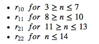
Dixon’s Q test [1] was “invented” as a convenient procedure to quickly identify outliers in datasets that only contains a small number of observations: typically 3 > n ≤ 10.
[1] R. B. Dean and W. J. Dixon (1951) Simplified Statistics for Small Numbers of Observations”. Anal. Chem., 1951, 23 (4), 636–638
Application
Although (at least in my opinion), the removal of outliers is a very questionable practice, this test is quite popular in the field of chemistry to “objectively” detect and reject outliers that are due to systematic errors by the experimentalist.
Criticism
If we want to use this test to legitimately remove (potential) outliers from a dataset, we should keep in mind that
- our data has to be normal distributed,
- and that we are not supposed to use this test more than once the same data set.
In my opinion, the Dixon Q-test should only be used with great caution, since this simple statistic is based on the assumption that the data is normal distributed, which can be quite challenging to predict for small sample sizes (if no prior/additional information is provided). Personally, I would use the Dixon Q-test to only detect outliers and not to remove those, which can help with the identification of uncertainties in the data set or problems in experimental procedures. Intuitively, this is quite similar to an approach of identifying samples that have a large standard deviation.
For example, if I tested ~1000 chemical compounds in some sort of activity assay - each compound 5 times, I would mark compounds that contain Q-test outliers for re-testing, because there might have been some problem in the measurement procedure that could have caused this inconsistency.
Method
1) Arrange values for observations in ascending order
First, we arrange the data for our sample in ascending order (from the lowest to the highest value):
\[x_1 \le x_2 \le . . . \le x_N\]2) Calculate Q
Next, we calculate the experimental Q-value (\(Q_{exp}\)).
Note that in a later paper in 1953, Dixon and Dean [3] revisited the calculation of the Q-value and reported different equations for different scenarios:
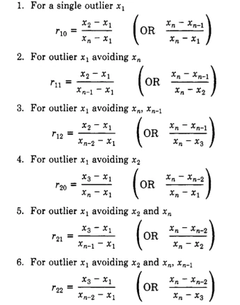
(from: Rorabacher, David B., 1991 [2])
However, according to a statement/observation in a more recent paper (Rorabacher, David B., 1991 [2]): “The \(r_{l0}\) ratio is commonly designated as ‘Q’ and is generally considered to be the most convenient, legitimate, statistical test available for the rejection of deviant values from a small sample conforming to a Gaussian distribution. (It is equally well suited to larger data sets if only one outlier is present.)”
Therefore, I will use \(r_{l0}\) for the following implementation of the Dixon Q-test:
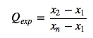
where it is assumed that the data is arranged in ascending order:
\[x_1 \le x_2 \le . . . \le x_N\][2] Rorabacher, David B. (1991) “Statistical Treatment for Rejection of Deviant Values: Critical Values of Dixon’s‘ Q’ Parameter and Related Subrange Ratios at the 95% Confidence Level.” Analytical Chemistry 63, no. 2 (1991): 139–46.
[3] W.J. Dixon: Processing data for outliers Reference”: J. Biometrics 9 (1953) 74-89
3) Compare the calculated to the tabulated critical Q-value
In the next step, we will compare the calculated \(Q_{exp}\) value to the to
the tabulated critical Q-value \(Q_{crit}\) for a chosen confidence
interval.
If the calculated Q-value for a particular observation is larger than
the critical Q-value (\(Q_{exp} \ge Q_{crit}\)), this observation is
considered to be an outlier according to the Q-test.
\(r_{10}\) Critical values for Dixon’s two-tailored Q-Test for 3 different confidence levels**
| N | Q90% | Q95% | Q99% |
|---|---|---|---|
| 3 | 0.941 | 0.97 | 0.994 |
| 4 | 0.765 | 0.829 | 0.926 |
| 5 | 0.642 | 0.71 | 0.821 |
| 6 | 0.56 | 0.625 | 0.74 |
| 7 | 0.507 | 0.568 | 0.68 |
| 8 | 0.468 | 0.526 | 0.634 |
| 9 | 0.437 | 0.493 | 0.598 |
| 10 | 0.412 | 0.466 | 0.568 |
| 11 | 0.392 | 0.444 | 0.542 |
| 12 | 0.376 | 0.426 | 0.522 |
| 13 | 0.361 | 0.41 | 0.503 |
| 14 | 0.349 | 0.396 | 0.488 |
| 15 | 0.338 | 0.384 | 0.475 |
| 16 | 0.329 | 0.374 | 0.463 |
| 17 | 0.32 | 0.365 | 0.452 |
| 18 | 0.313 | 0.356 | 0.442 |
| 19 | 0.306 | 0.349 | 0.433 |
| 20 | 0.3 | 0.342 | 0.425 |
| 21 | 0.295 | 0.337 | 0.418 |
| 22 | 0.29 | 0.331 | 0.411 |
| 23 | 0.285 | 0.326 | 0.404 |
| 24 | 0.281 | 0.321 | 0.399 |
| 25 | 0.277 | 0.317 | 0.393 |
| 26 | 0.273 | 0.312 | 0.388 |
| 27 | 0.269 | 0.308 | 0.384 |
| 28 | 0.266 | 0.305 | 0.38 |
| 29 | 0.263 | 0.301 | 0.376 |
| 30 | 0.26 | 0.29 | 0.372 |
4) Example
Let’s consider the following sample consisting of 5 observations:
0.142, 0.153, 0.135, 0.002, 0.175
- First, we sort it in ascending order: 0.002, 0.135, 0.142, 0.153, 0.175
- Next, we calculate the Q-value:
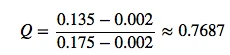
- Now, we look up the critical value for n=5 for a confidence level 95% in the Q-table \(= \ge 0.71\)
and we conclude that 0.002 (since 0.7687 > 0.71), that the observation 0.002 is an outlier at a confidence level of 95% according to Dixon’s Q-test.
Implementation
In the next few subsections, I will implement the Q-test in pure Python.
I have to apologize for not using packages from the sci-stack (pandas,
NumPy, scipy …) this time and thus making the code look less
elegant, but I wrote this code for a non-Python person and promised to
make it work with a standard Python installation.
Building dictionaries for Q-value look-up
We will build a simple set of dictionaries for different confidence intervals from the tabulated data in David B. Rorabacher’s paper: Rorabacher, David B. (1991) “Statistical Treatment for Rejection of Deviant Values: Critical Values of Dixon’s‘ Q’ Parameter and Related Subrange Ratios at the 95% Confidence Level.” Analytical Chemistry 63, no. 2 (1991): 139–46.
Then, we can use this dictionary to look up the critical Q-values (dictionary values) for different sample sizes (dictionary keys).
q90 = [0.941, 0.765, 0.642, 0.56, 0.507, 0.468, 0.437,
       0.412, 0.392, 0.376, 0.361, 0.349, 0.338, 0.329,
       0.32, 0.313, 0.306, 0.3, 0.295, 0.29, 0.285, 0.281,
       0.277, 0.273, 0.269, 0.266, 0.263, 0.26
      ]

q95 = [0.97, 0.829, 0.71, 0.625, 0.568, 0.526, 0.493, 0.466,
       0.444, 0.426, 0.41, 0.396, 0.384, 0.374, 0.365, 0.356,
       0.349, 0.342, 0.337, 0.331, 0.326, 0.321, 0.317, 0.312,
       0.308, 0.305, 0.301, 0.29
      ]

q99 = [0.994, 0.926, 0.821, 0.74, 0.68, 0.634, 0.598, 0.568,
       0.542, 0.522, 0.503, 0.488, 0.475, 0.463, 0.452, 0.442,
       0.433, 0.425, 0.418, 0.411, 0.404, 0.399, 0.393, 0.388,
       0.384, 0.38, 0.376, 0.372
       ]

Q90 = {n:q for n,q in zip(range(3,len(q90)+1), q90)}
Q95 = {n:q for n,q in zip(range(3,len(q95)+1), q95)}
Q99 = {n:q for n,q in zip(range(3,len(q99)+1), q99)}
Implementing a Dixon Q-test Function
Below, I wrote some simple Python code to test one data row for Dixon Q-test outliers:
def dixon_test(data, left=True, right=True, q_dict=Q95):
    """
    Keyword arguments:
        data = A ordered or unordered list of data points (int or float).
        left = Q-test of minimum value in the ordered list if True.
        right = Q-test of maximum value in the ordered list if True.
        q_dict = A dictionary of Q-values for a given confidence level,
            where the dict. keys are sample sizes N, and the associated values
            are the corresponding critical Q values. E.g.,
            {3: 0.97, 4: 0.829, 5: 0.71, 6: 0.625, ...}

    Returns a list of 2 values for the outliers, or None.
    E.g.,
       for [1,1,1] -> [None, None]
       for [5,1,1] -> [None, 5]
       for [5,1,5] -> [1, None]

    """
    assert(left or right), 'At least one of the variables, `left` or `right`, must be True.'
    assert(len(data) >= 3), 'At least 3 data points are required'
    assert(len(data) <= max(q_dict.keys())), 'Sample size too large'

    sdata = sorted(data)
    Q_mindiff, Q_maxdiff = (0,0), (0,0)

    if left:
        Q_min = (sdata[1] - sdata[0])
        try:
            Q_min /= (sdata[-1] - sdata[0])
        except ZeroDivisionError:
            pass
        Q_mindiff = (Q_min - q_dict[len(data)], sdata[0])

    if right:
        Q_max = abs((sdata[-2] - sdata[-1]))
        try:
            Q_max /= abs((sdata[0] - sdata[-1]))
        except ZeroDivisionError:
            pass
        Q_maxdiff = (Q_max - q_dict[len(data)], sdata[-1])

    if not Q_mindiff[0] > 0 and not Q_maxdiff[0] > 0:
        outliers = [None, None]

    elif Q_mindiff[0] == Q_maxdiff[0]:
        outliers = [Q_mindiff[1], Q_maxdiff[1]]

    elif Q_mindiff[0] > Q_maxdiff[0]:
        outliers = [Q_mindiff[1], None]

    else:
        outliers = [None, Q_maxdiff[1]]

    return outliers
Assertion Tests
Some simple assertion tests to make sure that the Dixon Q-test function behaves as expected/desired.
test_data1 = [0.142, 0.153, 0.135, 0.002, 0.175]
test_data2 = [0.542, 0.153, 0.135, 0.002, 0.175]

assert(dixon_test(test_data1) == [0.002, None]), 'expect [0.002, None]'
assert(dixon_test(test_data1, right=False) == [0.002, None]), 'expect [0.002, None]'
assert(dixon_test(test_data2) == [None, None]), 'expect [None, None]'
assert(dixon_test(test_data2, q_dict=Q90) == [None, 0.542]), 'expect [None, 0.542]'

print('ok')
ok
Example application
Below, I want to go through a naive example for our Dixon Q-test
function using an example CSV file.
In “real” application I would prefer NumPy and/or pandas, however
for this simple case the in-built Python csv library should suffice.
Below the example CSV file is shown that we are going to read in:
%%writefile ../../data/dixon_test_in.csv
,x1,x2,x3,x4,x5
id1,0.95,-0.65,0.6,0.82,NaN
id2,2.08,NaN,-1.43,0.38,NaN
id3,-0.46,NaN,-1.25,-2.62,0.22
id4,0.24,1.88,-0.49,-0.73,-0.49
id5,-1.65,2.1,-0.09,NaN,0.8
id6,-0.44,0.93,0.19,-4.36,-0.88
id7,0.36,-0.47,NaN,0.4,2.12
id8,1.29,-0.48,-0.6,-0.38,0.27
id9,-1.25,-1.35,1.13,1.7,-0.81
id10,0.04,1.98,NaN,NaN,NaN
import csv

def csv_to_list(csv_file, delimiter=','):
    """
    Reads in a CSV file and returns the contents as list,
    where every row is stored as a sublist, and each element
    in the sublist represents 1 cell in the table.

    """
    with open(csv_file, 'r') as csv_con:
        reader = csv.reader(csv_con, delimiter=delimiter)
        return list(reader)


def print_csv(csv_content):
    """ Prints CSV file to standard output."""
    print(50*'-')
    for row in csv_content:
        row = [str(e) for e in row]
        print('t'.join(row))
    print(50*'-')


def convert_cells_to_floats(csv_cont):
    """
    Converts cells to floats if possible
    (modifies input CSV content list).

    """
    for row in range(len(csv_cont)):
        for cell in range(len(csv_cont[row])):
            try:
                csv_cont[row][cell] = float(csv_cont[row][cell])
            except ValueError:
                pass
csv_cont = csv_to_list('../../data/dixon_test_in.csv')
convert_cells_to_floats(csv_cont)
print_csv(csv_cont)
--------------------------------------------------
    x1  x2  x3  x4  x5
id1 0.95    -0.65   0.6 0.82    nan
id2 2.08    nan -1.43   0.38    nan
id3 -0.46   nan -1.25   -2.62   0.22
id4 0.24    1.88    -0.49   -0.73   -0.49
id5 -1.65   2.1 -0.09   nan 0.8
id6 -0.44   0.93    0.19    -4.36   -0.88
id7 0.36    -0.47   nan 0.4 2.12
id8 1.29    -0.48   -0.6    -0.38   0.27
id9 -1.25   -1.35   1.13    1.7 -0.81
id10    0.04    1.98    nan nan nan
--------------------------------------------------
Now, let us add a new outlier column and apply the Dixon Q-test
function to our data set.
import math

csv_cont[0].append('outlier')

for row in csv_cont[1:]: # skips header
    nan_removed = [i for i in row[1:] if not math.isnan(i)]
    if len(nan_removed) >= 3:
        row.append(dixon_test(nan_removed, left=True, right=True, q_dict=Q90))
    else:
        row.append('NaN')
print_csv(csv_cont)

```python
--------------------------------------------------
    x1  x2  x3  x4  x5  outlier
id1 0.95    -0.65   0.6 0.82    nan [-0.65, None]
id2 2.08    nan -1.43   0.38    nan [None, None]
id3 -0.46   nan -1.25   -2.62   0.22    [None, None]
id4 0.24    1.88    -0.49   -0.73   -0.49   [None, None]
id5 -1.65   2.1 -0.09   nan 0.8 [None, None]
id6 -0.44   0.93    0.19    -4.36   -0.88   [-4.36, None]
id7 0.36    -0.47   nan 0.4 2.12    [None, None]
id8 1.29    -0.48   -0.6    -0.38   0.27    [None, None]
id9 -1.25   -1.35   1.13    1.7 -0.81   [None, None]
id10    0.04    1.98    nan nan nan NaN
--------------------------------------------------
As we can see in the table above, we have 2 potential outliers in our data set. Finally, we let us write the results to a new CSV file for future reference:
def write_csv(dest, csv_cont):
    """ Writes a comma-delimited CSV file. """

    with open(dest, 'w') as out_file:
        writer = csv.writer(out_file, delimiter=',')
        for row in csv_cont:
            writer.writerow(row)

write_csv('../../data/dixon_test_out.csv', csv_cont)
Plotting the Data
To get a visual impression of how our data looks like, let us make some simple plots.
Bar plot of the sample means with standard deviation
First, let’s create a bar plot with standard deviation, since such bar plots with standard deviation or standard error bars are probably the most common plots in any field. Although it is not always appropriate it is certainly the kind of data visualization we are most familiar with - due to the frequent exposure when reading scientific research articles.
import numpy as np
from matplotlib import pyplot as plt

all_means = [np.nanmean(row[1:6]) for row in csv_cont[1:]]
all_stddevs = [np.nanstd(row[1:6]) for row in csv_cont[1:]]

fig = plt.figure(figsize=(8,6))

y_pos = np.arange(len(csv_cont[1:]))
y_pos = [x for x in y_pos]
plt.yticks(y_pos, [row[0] for row in csv_cont[1:]], fontsize=10)
plt.xlabel('measurement x')
t = plt.title('Bar plot with standard deviation')

plt.grid()
plt.barh(y_pos, all_means, xerr=all_stddevs, align='center', alpha=0.4, color='g')

plt.show()
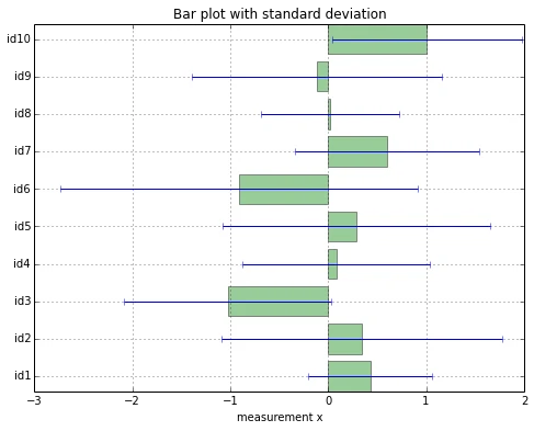
As we would expect, basically every sample has a very (relatively) large standard deviation. However, we can’t derive any detail about a possible cause for this large deviation: whether it is just due to 1 outlier, or if the whole data widely spread in general.
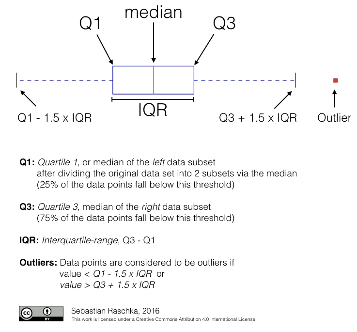
Boxplot
A more useful plot in my opinion is Tukey’s boxplot [4]. Boxplots are in facts one of my preferred approaches to quickly and visually indicate outliers in a Gaussian data set. However, also boxplots have to be used with real caution and might also not very informative for small sample sizes.
[4] Robert McGill, John W. Tukey and Wayne A. Larsen: “The American Statistician” Vol. 32, No. 1 (Feb., 1978), pp. 12-16
csv_nonan = [[x for x in row[1:6] if not math.isnan(x)] for row in csv_cont[1:]]
fig = plt.figure(figsize=(8,6))
plt.boxplot(csv_nonan,0,'rs',0)
plt.yticks([y+1 for y in y_pos], [row[0] for row in csv_cont[1:]])
plt.xlabel('measurement x')
t = plt.title('Box plot')
plt.show()
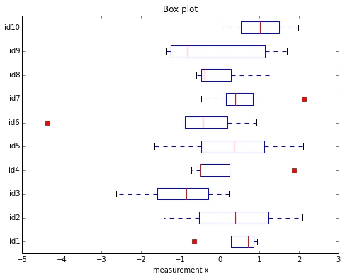
The red squares indicate the outliers here. Quite interestingly, both outliers for the samples “id6” and “id1” where also picked up in our previous Dixon Q-test. However, the outliers in “id4” and “id7” were not indicated as outliers by Dixon’s outlier test.
Conclusion
I really don’t want to draw any conclusion about which approach is right or wrong here, since in my opinion, drawing any conclusion from a data set that is based on such a small number of observations simply just doesn’t make sense!
So you may wonder why I wasted your time if you read this article up to this point? Since Dixon’s Q-test is still quite popular in certain scientific fields (e.g., chemistry) that it is important to understand its principles in order to draw your own conclusion of the presented research data that you might stumble upon in research articles or scientific talks.
Read Next
 Scientific Computing in Python: Introduction to NumPy and Matplotlib
Beginner's guide to NumPy and Matplotlib for scientific computing: arrays, indexing, broadcasting, linear algebra, and plotting with Python code examples.
Scientific Computing in Python: Introduction to NumPy and Matplotlib
Beginner's guide to NumPy and Matplotlib for scientific computing: arrays, indexing, broadcasting, linear algebra, and plotting with Python code examples.
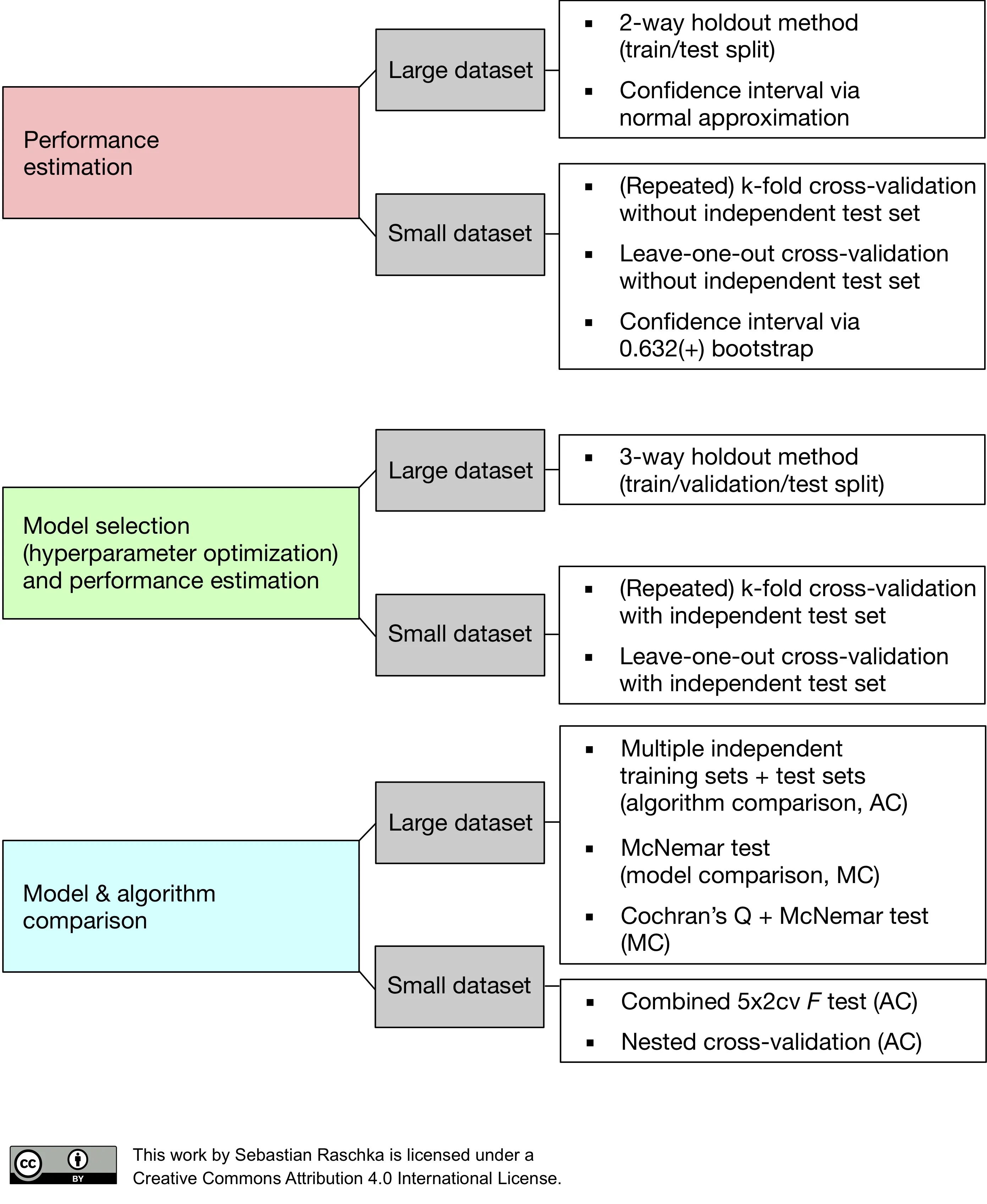 Model evaluation, model selection, and algorithm selection in machine learning
Part 4 of the model evaluation series explaining statistical tests, algorithm comparisons, corrected resampled tests, and nested cross-validation.
Model evaluation, model selection, and algorithm selection in machine learning
Part 4 of the model evaluation series explaining statistical tests, algorithm comparisons, corrected resampled tests, and nested cross-validation.
 Generating Gender-Neutral Face Images with Semi-Adversarial Neural Networks to Enhance Privacy
I thought that it would be nice to have short and concise summaries of recent projects handy, to share them with a more general audience, including...
Generating Gender-Neutral Face Images with Semi-Adversarial Neural Networks to Enhance Privacy
I thought that it would be nice to have short and concise summaries of recent projects handy, to share them with a more general audience, including...

If you read the book and have a few minutes to spare, I'd really appreciate a brief review. It helps us authors a lot!
Your support means a great deal! Thank you!