Machine Learning FAQ
What is the relationship between deep learning and regular machine learning on a conceptual level?
That’s an interesting question, and I try to answer this is a very general way.
In essence, deep learning offers a set of techniques and algorithms that help us to parameterize deep neural network structures – artificial neural networks with many hidden layers and parameters. One of the key ideas behind deep learning is to extract high level features from the given dataset. Thereby, deep learning aims to overcome the challenge of the often tedious feature engineering task and helps with parameterizing traditional neural networks with many layers.
Now, to introduce deep learning, let us take a look at a more concrete example involving multi-layer perceptrons (MLPs):
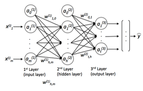
On a tangent: The term “perceptron” in MLPs may be a bit confusing since we don’t really want only linear neurons in our network. Using MLPs, we want to learn complex functions to solve non-linear problems. Thus, our network is conventionally composed of one or multiple “hidden” layers that connect the input and output layer. Those hidden layers normally have some sort of sigmoid activation function (log-sigmoid or the hyperbolic tangent etc.). For example, think of a log-sigmoid unit in our network as a logistic regression unit that returns continuous values outputs in the range 0-1. A simple MLP could look like this

where y_hat is the final class label that we return as the prediction based on the inputs (x) if this are classification tasks. The “a”s are our activated neurons and the “w”s are the weight coefficients. Now, if we add multiple hidden layers to this MLP, we’d also call the network “deep.” The problem with such “deep” networks is that it becomes tougher and tougher to learn “good” weights for this network. When we start training our network, we typically assign random values as initial weights, which can be terribly off from the “optimal” solution we want to find. During training, we then use the popular backpropagation algorithm (think of it as reverse-mode auto-differentiation) to propagate the “errors” from right to left and calculate the partial derivatives with respect to each weight to take a step into the opposite direction of the cost (or “error”) gradient. Now, the problem with deep neural networks is the so-called “vanishing gradient” – the more layers we add, the harder it becomes to “update” our weights because the signal becomes weaker and weaker. Since our network’s weights can be terribly off in the beginning (random initialization) it can become almost impossible to parameterize a “deep” neural network with backpropagation.
Deep Learning
Now, this is where “deep learning” comes into play. Roughly speaking, we can think of deep learning as “clever” tricks or algorithms that can help we with the training of such “deep” neural network structures. There are many, many different neural network architectures, but to continue with the example of the MLP, let me introduce the idea of convolutional neural networks (ConvNets). We can think of those as an “add-on” to our MLP that helps we to detect features as “good” inputs for our MLP.
In applications of “usual” machine learning, there is typically a strong focus on the feature engineering part; the model learned by an algorithm can only be so good as its input data. Of course, there must be sufficient discriminatory information in our dataset, however, the performance of machine learning algorithms can suffer substantially when the information is buried in meaningless features. The goal behind deep learning is to automatically learn the features from (somewhat) noisy data; it’s about algorithms that do the feature engineering for us to provide deep neural network structures with meaningful information so that it can learn more effectively. We can think of deep learning as algorithms for automatic “feature engineering,” or we could simply call them “feature detectors,” which help us to overcome the vanishing gradient challenge and facilitate the learning in neural networks with many layers.
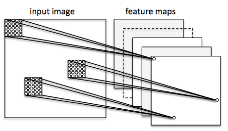
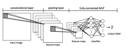
Let’s consider a ConvNet in context of image classification. Here, we use so-called “receptive fields” (think of them as “windows”) that slide over our image. We then connect those “receptive fields” (for example of the size of 5x5 pixel) with 1 unit in the next layer, this is the so-called “feature map.” After this mapping, we have constructed a so-called convolutional layer. Note that our feature detectors are basically replicates of one another – they share the same weights. The idea is that if a feature detector is useful in one part of the image, it is likely that it is useful somewhere else, but at the same time it allows each patch of image to be represented in several ways.

Next, we have a “pooling” layer, where we reduce neighboring features from our feature map into single units (by taking the max feature or by averaging them, for example). We do this over many rounds and eventually arrive at an almost scale invariant representation of our image (the exact term is “equivariant”). This is very powerful since we can detect objects in an image no matter where they are located.

In essence, the “convolutional” add-on that acts as a feature extractor or filter to our MLP. Via the convolutional layers we aim to extract the useful features from the images, and via the pooling layers, we aim to make the features somewhat equivariant to scale and translation.
If you like this content and you are looking for similar, more polished Q & A’s, check out my new book Machine Learning Q and AI.