Model evaluation, model selection, and algorithm selection in machine learning
Part IV - Comparing the performance of machine learning models and algorithms using statistical tests and nested cross-validation
A single-PDF version of Model Evaluation parts 1-4 is available on arXiv: https://arxiv.org/abs/1811.12808
Introduction
This final article in the series Model evaluation, model selection, and algorithm selection in machine learning presents overviews of several statistical hypothesis testing approaches, with applications to machine learning model and algorithm comparisons. This includes statistical tests based on target predictions for independent test sets (the downsides of using a single test set for model comparisons was discussed in previous articles) as well as methods for algorithm comparisons by fitting and evaluating models via cross-validation. Lastly, this article will introduce nested cross-validation, which has become a common and recommended a method of choice for algorithm comparisons for small to moderately-sized datasets.
Then, at the end of this article, I provide a list of my personal suggestions concerning model evaluation, selection, and algorithm selection summarizing the several techniques covered in this series of articles.
Testing the Difference of Proportions
There are several different statistical hypothesis testing frameworks that are being used in practice to compare the performance of classification models, including conventional methods such as difference of two proportions (here, the proportions are the estimated generalization accuracies from a test set), for which we can construct 95% confidence intervals based on the concept of the Normal Approximation to the Binomial that was covered in Part I.
Performing a z-score test for two population proportions is inarguably the most straight-forward way to compare to models (but certainly not the best!): In a nutshell, if the 95% confidence intervals of the accuracies of two models do not overlap, we can reject the null hypothesis that the performance of both classifiers is equal at a confidence level of \(\alpha=0.05\) (or 5% probability). Violations of assumptions aside (for instance that the test set samples are not independent), as Thomas Dietterich noted based on empirical results in a simulated study (Dietterich 1998), this test tends to have a high false positive rate (here: incorrectly detecting difference when there is none), which is among the reasons why it is not recommended in practice.
Nonetheless, for the sake of completeness, and since it a commonly used method in practice, the general procedure is outlined below as follows (which also generally applies to the different hypothesis tests presented later):
- formulate the hypothesis to be tested (for instance, the null hypothesis stating that the proportions are the same; consequently, the alternative hypothesis that the proportions are different, if we use a two-tailed test);
- decide upon a significance threshold (for instance, if the probability of observing a difference more extreme than the one seen is more than 5%, then we plan to reject the null hypothesis);
- analyze the data, compute the test statistic (here: z-score), and compare its associated p-value (probability) to the previously determined significance threshold;
- based on the p-value and significance threshold, either accept or reject the null hypothesis at the given confidence level and interpret the results.
The z-score is computed as the observed difference divided by the square root for their combined variances
\[z = \frac{ACC_1 - ACC_2}{\sqrt{\sigma_{1}^2 + \sigma_{2}^2}},\]where \(ACC_1\) is the accuracy of one model and \(ACC_2\) is the accuracy of a second model estimated from the test set. Recall that we computed the variance of the estimated accuracy as
\[\sigma^2 = \frac{ACC(1-ACC)}{n}\]in Part I and then computed the confidence interval (Normal Approximation Interval) as
\[ACC \pm z \times \sigma,\]where \(z=1.96\) for a 95% confidence interval. Comparing the confidence intervals of two accuracy estimates and checking whether they overlap is then analogous to computing the \(z\) value for the difference in proportions and comparing the probability (p-value) to the chosen significance threshold. So, to compute the z-score directly for the difference of two proportions, \(ACC_1\) and \(ACC_2\), we pool these proportions (assuming that \(ACC_1\) and \(ACC_2\) are the performances of two models estimated on two indendent test sets of size \(n_1\) and \(n_2\), respectively),
\[ACC_{1, 2} = \frac{ACC_1 \times n_1 + ACC_2 \times n_2}{n_1 + n_2},\]and compute the standard deviation as
\[\sigma_{1,2} = \sqrt{ ACC_{1,2} (1-ACC_{1,2}) \times \left(\frac{1}{n_1} + \frac{1}{n_2}\right) },\]such that we can compute the z-score,
\[z = \frac{ACC_1 - ACC_2}{\sigma_{1,2}}.\]Since, due to using the same test set (and violating the independence assumption) we have \(n_1 = n_2 = n\), so that we can simplify the z-score computation to
\[z = \frac{ACC_1 - ACC_2}{\sqrt{2\sigma^2}} = \frac{ACC_1 - ACC_2}{\sqrt{2\cdot ACC_{1,2}(1-ACC_{1,2}))/n}},\]where \(ACC_{1, 2}\) is simply \((ACC_1 + ACC_2)/2\).
In the second step, based on the computed \(z\) value (this assumes the test errors are independent, which is usually violated in practice as we use the same test set) we can reject the null hypothesis that the pair of models has equal performance (here, measured in “classification accuracy”) at an \(\alpha=0.05\) level if \(\lvert z \rvert\) is higher than 1.96. Alternatively, if we want to put in the extra work, we can compute the area under the standard normal cumulative distribution at the z-score threshold. If we find this p-value is smaller than a significance level we set before conducting the test, then we can reject the null hypothesis at that given significance level.
The problem with this test though is that we use the same test set to compute the accuracy of the two classifiers; thus, it might be better to use a paired test such as a paired sample t-test, but a more robust alternative is the McNemar test illustrated in the next section.
Comparing Two Models with the McNemar Test
So, instead of using the “difference of proportions” test, Dietterich (Dietterich, 1998) found that the McNemar test is to be preferred. The McNemar test, introduced by Quinn McNemar in 1947 (McNemar 1947), is a non-parametric statistical test for paired comparisons that can be applied to compare the performance of two machine learning classifiers.
Often, McNemar’s test is also referred to as “within-subjects chi-squared test,” and it is applied to paired nominal data based on a version of 2x2 confusion matrix (sometimes also referred to as 2x2 contingency table) that compares the predictions of two models to each other (not be confused with the typical confusion matrices encountered in machine learning, which are listing false positive, true positive, false negative, and true negative counts of a single model). The layout of the 2x2 confusion matrix suitable for McNemar’s test is shown in the following figure:
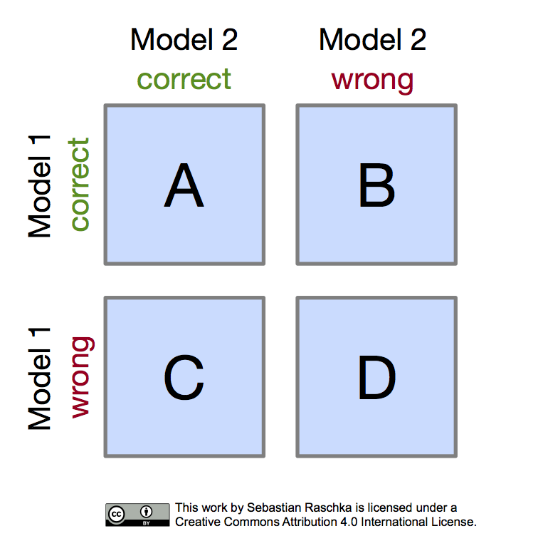
Given such a 2x2 confusion matrix as shown in the previous figure, we can compute the accuracy of a Model 1 via \((A+B) / (A+B+C+D)\), where \(A+B+C+D\) is the total number of test examples \(n\). Similarly, we can compute the accuracy of Model 2 as \((A+C) / n\). The most interesting numbers in this table are in cells B and C, though, as A and D merely count the number of samples where both Model 1 and Model 2 made correct or wrong predictions, respectively. Cells B and C (the off-diagonal entries), however, tell us how the models differ. To illustrate this point, let us take a look at the following example:
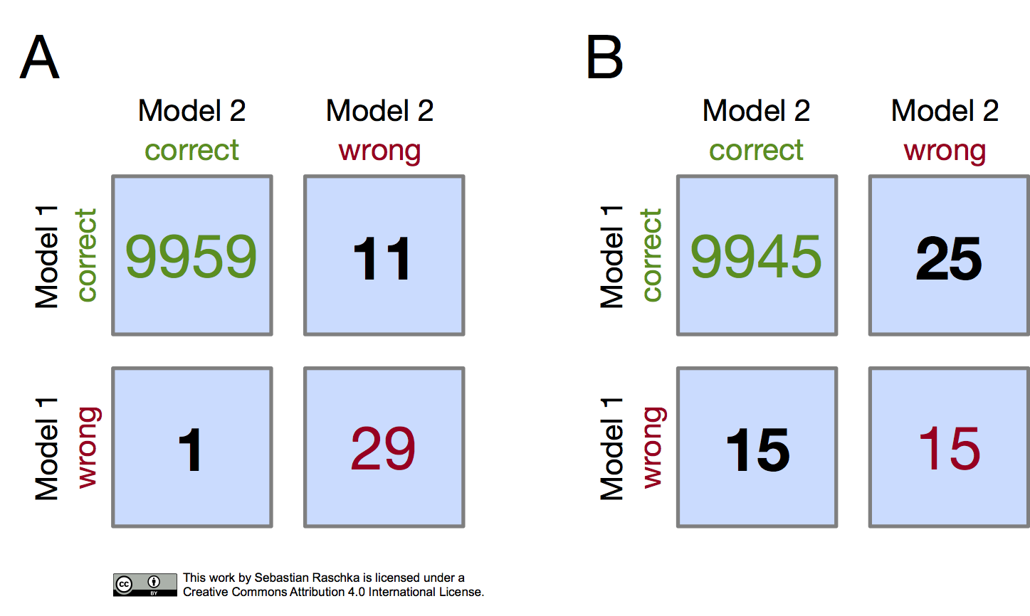
In both subpanels, A and B, the accuracy of Model 1 and Model 2 are 99.6% and 99.7%, respectively.
- Model 1 accuracy subpanel A: \((9959+11) / 10000 \times 100\% = 99.7\%\)
- Model 1 accuracy subpanel B: \((9945+25) / 10000 \times 100\% = 99.7\%\)
- Model 2 accuracy subpanel A: \((9959+1) / 10000 \times 100\% = 99.6\%\)
- Model 2 accuracy subpanel B: \((9945+15) / 10000 \times 100\% = 99.6\%\)
Now, in subpanel A, we can see that Model 1 got 11 predictions right that Model 2 got wrong. Vice versa, Model 2 got one prediction right that Model 1 got wrong. Thus, based on this 11:1 ratio, we may conclude, based on our intuition, that Model 1 performs substantially better than Model 2. However, in subpanel B, the Model 1:Model 2 ratio is 25:15, which is less conclusive about which model is the better one to choose. This is a good example where McNemar’s test can come in handy.
In McNemar’s Test, we formulate the null hypothesis that the probabilities \(p(B)\) and \(p(C)\) – where \(B\) and \(C\) refer to the confusion matrix cells introduced in an earlier figure – are the same, or in simplified terms: None of the two models performs better than the other. Thus, we might consider the alternative hypothesis that the performances of the two models are not equal.
The McNemar test statistic (“chi-squared”) can be computed as follows:
\[\chi^2 = \frac{(B-C)^2}{B+C}.\]After setting a significance threshold, for example, \(\alpha=0.05\), we can compute a p-value – assuming that the null hypothesis is true, the p-value is the probability of observing the given empirical (or a larger) \(\chi^2\)-squared value. If the p-value is lower than our chosen significance level, we can reject the null hypothesis that the two models’ performances are equal.
Since the McNemar test statistic, \(\chi^2\), follows a \(\chi^2\) distribution with one degree of freedom (assuming the null hypothesis and relatively large numbers in cells B and C, say > 25), we can now use our favorite software package to “look up” the (1-tail) probability via the \(\chi^2\) probability distribution with one degree of freedom.
If we did this for scenario B in the previous figure (\(\chi^2=2.5\)), we would obtain a p-value of 0.1138, which is larger than our significance threshold, and thus, we cannot reject the null hypothesis. Now, if we computed the p-value for scenario A (\(\chi^2=8.3\)), we would obtain a p-value of 0.0039, which is below the set significance threshold (\(\alpha=0.05\)) and leads to the rejection of the null hypothesis; we can conclude that the models’ performances are different (for instance, Model 1 performs better than Model 2).
Approximately one year after Quinn McNemar published the McNemar Test (McNemar 1947), Allen L. Edwards (Edwards 1948) proposed a continuity corrected version, which is the more commonly used variant today:
\[\chi^2 = \frac{\big(| B - C| -1 \big)^2}{B+C}.\]In particular, Edwards wrote:
This correction will have the apparent result of reducing the absolute value of the difference, [B - C], by unity.
According to Edwards, this continuity correction increases the usefulness and accuracy of McNemar’s test if we are dealing with discrete frequencies and the data is evaluated regarding the chi-squared distribution.
A function for using McNemar’s test is implemented in MLxtend (Raschka, 2018): http://rasbt.github.io/mlxtend/user_guide/evaluate/mcnemar/.
Exact p-values via the Binomial Test
While McNemar’s test approximates the p-values reasonably well if the values in cells B and C are larger than 50 (referring to the 2x2 confusion matrix shown earlier), for example, it makes sense to use a computationally more expensive binomial test to compute the exact p-values if the values of B and C are relatively small – since the chi-squared value from McNemar’s test may not be well-approximated by the chi-squared distribution.
The exact p-value can be computed as follows (based on the fact that McNemar’s test, under the null hypothesis, is essentially a binomial test with proportion 0.5):
\[p = 2 \sum^{n}_{i=max(B, C)} \binom{n}{i} 0.5^i (1 - 0.5)^{n-i},\]where \(n=B+C\), and the factor 2 is used to compute the two-sided p-value (here, \(n\) is not to be confused with the test set size \(n\)).
The following heat map illustrates the differences between the McNemar approximation of the chi-squared value (with and without Edward’s continuity correction) to the exact p-values computed via the binomial test:
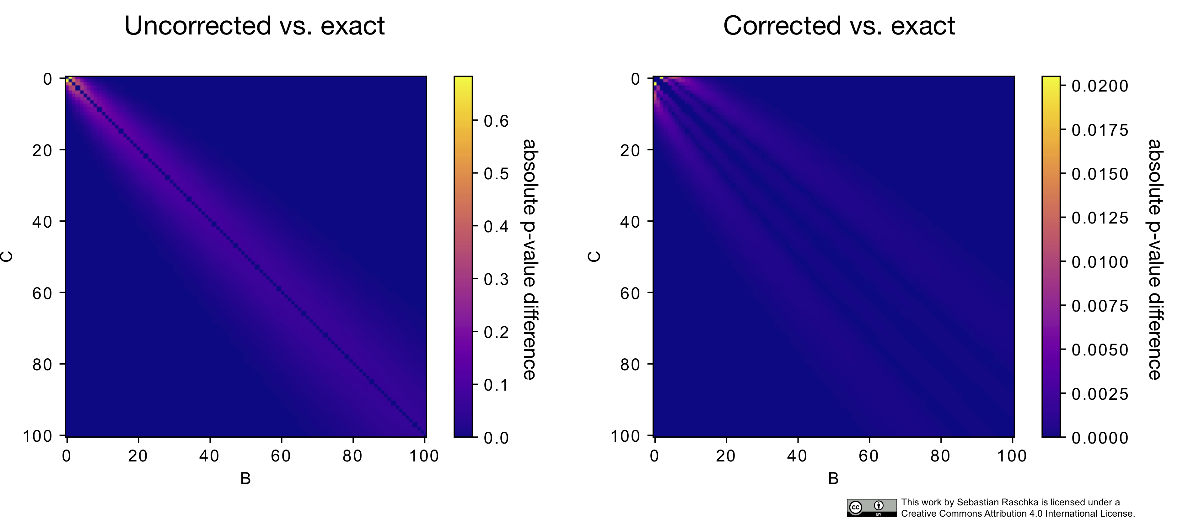
As we can see in this heat map above, the p-values from the continuity-corrected version of McNemar’s test are almost identical to the p-values from a binomial test if both B and C are larger than 50. (The MLxtend function, mcnemar, provides different options for toggling between the regular and the corrected McNemar test as well as including an option to compute the exact p-values, http://rasbt.github.io/mlxtend/user_guide/evaluate/mcnemar/)
Multiple Hypotheses Testing
In the previous section, we discussed how we could compare two machine learning classifiers using McNemar’s test. However, in practice, we often have more than two models that we like to compare based on their estimated generalization performance – for instance, the predictions on an independent test set. Now, applying the testing procedure described earlier multiple times will result in a typical issue called “multiple hypotheses testing.” A common approach for dealing with such scenarios is the following:
- Conduct an omnibus test under the null hypothesis that there is no difference between the classification accuracies.
- If the omnibus test led to the rejection of the null hypothesis, conduct pairwise post hoc tests, with adjustments for multiple comparisons, to determine where the differences between the model performances occurred. (Here, we could use McNemar’s test, for example.)
Omnibus tests are statistical tests designed to check whether random samples depart from a null hypothesis. A popular example of an omnibus test is the so-called Analysis of Variance (ANOVA), which is a procedure for analyzing the differences between group means. Alternatively, in other words, ANOVA is commonly used for testing the significance of the null hypothesis that the means of several groups are equal. To compare multiple machine learning models, Cochran’s Q test would be a possible choice, which is essentially a generalized version of McNemar’s test for three or more models. However, omnibus tests are overall significance tests that do not provide information about how the different models differ – omnibus tests such as Cochran’s Q only tell us that a group of models differs or not.
Since omnibus tests can tell us that but not how models differ, we can perform post hoc tests if an omnibus test leads to the rejection of the null hypothesis. Alternatively, in other words, if we successfully rejected the null hypothesis that the performance of three or models is the same at a predetermined significance threshold, we may conclude that there is at least one significant difference among the different models.
By definition, post hoc testing procedures do not require any “prior” plan for testing. Hence, post hoc testing procedures may have a bad reputation and may be regarded as “fishing expeditions” or “searching for the needle in the haystack,” because no hypothesis is clear beforehand in terms of which models should be compared, so that it is required to compare all possible pairs of models with each other, which leads to the multiple hypothesis problems that we briefly discussed in Part III. However, please keep in mind that these are all approximations and everything concerning statistical tests and reusing test sets (independence violation) should be taken with (at least) a grain of salt.
For the post hoc procedure, we could use one of the many correction terms, for example, Bonferroni’s correction (Bonferroni, 1936; Dunn 1961) for multiple hypothesis testing. In a nutshell, where a given significance threshold (or \(\alpha\)-level) may be appropriate for a single comparison between to models, it is not suitable for multiple pair-wise comparisons. For instance, using the Bonferroni correction is a means to reduce the false positive rate in multiple comparison tests by adjusting the significance threshold to be more conservative.
The next two sections will discuss two omnibus tests, Cochran’s Q test and the F-test for comparing multiple classifiers on the same test set proposed by Looney (Looney, 1988).
Cochran’s Q Test for Comparing the Performance of Multiple Classifiers
Cochran’s Q test can be regarded as a generalized version of McNemar’s test that can be applied to compare three or more classifiers. In a sense, Cochran’s Q test is similar to ANOVA but for paired nominal data. Similar to ANOVA, it does not provide us with information about which groups (or models) differ – only tells us that there is a difference among the models.
The test statistic \(Q\) is approximately, (similar to McNemar’s test), distributed as chi-squared with \(M-1\) degrees of freedom, where \(M\) is the number of models we evaluate (since \(M=2\) for McNemar’s test, McNemar’s test statistic approximates a chi-squared distribution with one degree of freedom).
More formally, Cochran’s Q test tests the null hypothesis (\(H_0\)) that there is no difference between the classification accuracies (Fleiss, 2013):
\[H_0: ACC_1 = ACC_2 = \ldots = ACC_M.\]Let \(\{C_1, \dots , C_M\}\) be a set of classifiers who have all been tested on the same dataset. If the \(M\) classifiers do not differ in terms of their performance, then the following \(Q\) statistic is distributed approximately as “chi-squared” with \(M-1\) degrees of freedom:
\[Q = (M-1) \frac{M \sum^{M}_{i=1}G_{i}^{2} - T^2}{MT - \sum^{n}_{j=1}M_j^2} .\]Here, \(G_i\) is the number of objects out of the \(n\) test examples correctly classified by \(C_i= 1, \dots M\); \(M_j\) is the number of classifiers out of \(M\) that correctly classified the \(j\)th example in the test dataset; and \(T\) is the total number of correct number of votes among the \(M\) classifiers (Kuncheva, 2004):
\[T = \sum_{i=1}^{M}; \quad G_i = \sum^{N}_{j=1} M_j.\]To perform Cochran’s Q test, we typically organize the classifier predictions in a binary \(n \times M\) matrix (number of test examples vs. the number of classifiers). The \(ij\text{th}\) entry of such matrix is 0 if a classifier \(C_j\) has misclassified a data example (vector) \(\mathbf{x}_i\) and 1 otherwise (if the classifier predicted the class label \(f(\mathbf{x}_i)\) correctly).
Applied to an example dataset that was taken from (Kuncheva, 2004), the procedure below illustrates how the classification results may be organized. For instance, assume we have the ground truth labels of the test dataset \(\mathbf{y}_{true}\)
and the following predictions on the test set by 3 classifiers (\(\mathbf{y}_{C_1}\), \(\mathbf{y}_{C_2}\), and \(\mathbf{y}_{C_3}\)):
\[\mathbf{y}_{true} = [0, 0, 0, 0, 0, 0, 0, 0, 0, 0, 0, 0, 0, 0, 0, 0, 0, 0, 0, 0,\\ 0, 0, 0, 0, 0, 0, 0, 0, 0, 0, 0, 0, 0, 0, 0, 0, 0, 0, 0, 0, \\ 0, 0, 0, 0, 0, 0, 0, 0, 0, 0, 0, 0, 0, 0, 0, 0, 0, 0, 0, 0, \\ 0, 0, 0, 0, 0, 0, 0, 0, 0, 0, 0, 0, 0, 0, 0, 0, 0, 0, 0, 0,\\ 0, 0, 0, 0, 0, 0, 0, 0, 0, 0, 0, 0, 0, 0, 0, 0, 0, 0, 0, 0];\] \[\mathbf{y}_{C_1} = [1, 1, 1, 1, 1, 1, 1, 1, 1, 1, 1, 1, 1, 1, 1, 1, 0, 0, 0, 0,\\ 0, 0, 0, 0, 0, 0, 0, 0, 0, 0, 0, 0, 0, 0, 0, 0, 0, 0, 0, 0,\\ 0, 0, 0, 0, 0, 0, 0, 0, 0, 0, 0, 0, 0, 0, 0, 0, 0, 0, 0, 0,\\ 0, 0, 0, 0, 0, 0, 0, 0, 0, 0, 0, 0, 0, 0, 0, 0, 0, 0, 0, 0,\\ 0, 0, 0, 0, 0, 0, 0, 0, 0, 0, 0, 0, 0, 0, 0, 0, 0, 0, 0, 0];\] \[\mathbf{y}_{C_2} = [1, 1, 1, 1, 1, 1, 0, 0, 0, 0, 0, 0, 0, 0, 0, 0, 0, 0, 0, 0,\\ 1, 1, 0, 0, 0, 0, 0, 0, 0, 0, 0, 0, 0, 0, 0, 0, 0, 0, 0, 0,\\ 0, 0, 0, 0, 0, 0, 0, 0, 0, 0, 0, 0, 0, 0, 0, 0, 0, 0, 0, 0,\\ 0, 0, 0, 0, 0, 0, 0, 0, 0, 0, 0, 0, 0, 0, 0, 0, 0, 0, 0, 0,\\ 0, 0, 0, 0, 0, 0, 0, 0, 0, 0, 0, 0, 0, 0, 0, 0, 0, 0, 0, 0];\] \[\mathbf{y}_{C_3} = [1, 1, 1, 0, 0, 0, 1, 0, 0, 0, 0, 0, 0, 0, 0, 0, 0, 0, 0, 0,\\ 1, 1, 0, 0, 0, 0, 0, 0, 0, 0, 0, 0, 0, 0, 0, 0, 0, 0, 0, 0,\\ 0, 0, 0, 0, 0, 0, 0, 0, 0, 0, 0, 0, 0, 0, 0, 0, 0, 0, 0, 0,\\ 0, 0, 0, 0, 0, 0, 0, 0, 0, 0, 0, 0, 0, 0, 0, 0, 0, 0, 0, 0,\\ 0, 0, 0, 0, 0, 0, 0, 0, 0, 0, 0, 0, 0, 0, 0, 0, 0, 0, 1, 1].\]We can then tabulate the correct (1) and incorrect (0) classifications as follows:
| \(C_1\) (model 1) | \(C_2\) (model 2) | \(C_3\) (model 3) | Occurrences | |
|---|---|---|---|---|
| 1 | 1 | 1 | 80 | |
| 1 | 1 | 0 | 2 | |
| 1 | 0 | 1 | 0 | |
| 1 | 0 | 0 | 2 | |
| 0 | 1 | 1 | 9 | |
| 0 | 1 | 0 | 1 | |
| 0 | 0 | 1 | 3 | |
| 0 | 0 | 0 | 3 | |
| Accuracy | \(84/100 \times 100\% = 84\%\) | \(92/100 \times 100\% = 92\%\) | \(92/100 \times 100\% = 92\%\) |
By plugging in the respective value into the previous equation, we obtain the following \(Q\) value:
\[Q = 2 \times \frac{3 \times (84^2 + 92^2 + 92^2) - 268^2}{3\times 268-(80 \times 9 + 11 \times 4 + 6 \times 1)} \approx 7.5294.\]Now, the Q value (approximating \(\chi^2\)) corresponds to a p-value of approximately 0.023 assuming a \(\chi^2\) distribution with \(M-1 = 2\) degrees of freedom. Assuming that we chose a significance level of \(\alpha=0.05\), we would reject the null hypothesis that all classifiers perform equally well, since \(0.023 < \alpha\). (An implementation of Cochran’s Q test is provided in MLxtend, http://rasbt.github.io/mlxtend/user_guide/evaluate/cochrans_q/.)
In practice, if we successfully rejected the null hypothesis, we could perform multiple post hoc pair-wise tests – for example, McNemar’s test with a Bonferroni correction – to determine which pairs have different population proportions. Unfortunately, numerous comparisons are usually very tricky in practice. Peter H. Westfall, James F. Troendl, and Gene Pennello wrote a nice article on how to approach such situations where we want to compare multiple models to each other (Westfall and others 2010).
As Perneger, Thomas V (Perneger, 1998) writes:
Type I errors [False Positives] cannot decrease (the whole point of Bonferroni adjustments) without inflating type II errors (the probability of accepting the null hypothesis when the alternative is true) (Rothman, 1990). And type II errors [False Negatives] are no less false than type I errors.
Eventually, once more it comes down to the “no free lunch” – in this context, let us refer of it as the “no free lunch theorem of statistical tests.” However, statistical testing frameworks can be a valuable aid in decision making. So, in practice, if we are honest and rigorous, the process of multiple hypothesis testing with appropriate corrections can be a crucial aid in decision making. However, we have to be careful that we do not put too much emphasis on such procedures when it comes to assessing evidence in data.
The F-Test for Comparing Multiple Classifiers
Almost ironically, Cochran noted that in his work on the Q test (Cochran, 1950)
If the data had been measured variables that appeared normally distributed, instead of a collection of 1’s and 0’s, the F-test would be almost automatically applied as the appropriate method. Without having looked into that matter, I had once or twice suggested to research workers that the F-test might serve as an approximation even when the table consists of 1’s and 0’s
The method of using the F-test for comparing two classifiers in this section is somewhat loosely based on Looney, 1988, (whereas it shall be noted that Looney recommends an adjusted version called \(F^+\) test).
In the context of the F-test, our null hypothesis is again that there that there is no difference between the classification accuracies:
\[p_i: H_0 = p_1 = p_2 = \cdots = p_L.\]Let \(\{C_1, \dots , C_M\}\) be a set of classifiers which have all been tested on the same dataset. If the \(M\) classifiers do not perform differently, then the F statistic is distributed according to an F distribution with \((M-1)\) and \((M-1)\times n\) degrees of freedom, where \(n\) is the number of examples in the test set. The calculation of the F statistic consists of several components, which are listed below (adopted from \cite{looney1988statistical}).
We start by defining \(ACC_{avg}\) as the average of the accuracies of the different models
\[ACC_{avg} = \frac{1}{M}\sum_{j=1}^M ACC_j.\]The sum of squares of the classifiers is then computed as
\[SSA = n \sum_{j=1}^{M} (G_j)^2 -n \cdot M \cdot ACC_{avg},\]where $G_j$ is the proportion of the \(n\) examples classified correctly by classifier \(j\).
The sum of squares for the objects is calculated as follows:
\[SSB= \frac{1}{M} \sum_{j=1}^n (M_j)^2 - M\cdot n \cdot ACC_{avg}^2.\]Here, \(M_j\) is the number of classifiers out of $M$ that correctly classified object \(\mathbf{x}_j \in \mathbf{X}_{n}\), where \(\mathbf{X}_{n} = \{\mathbf{x}_1, ... \mathbf{x}_{n}\}\) is the test dataset on which the classifiers are tested on.
Finally, we compute the total sum of squares,
\[SST = M\cdot n \cdot ACC_{avg} (1 - ACC_{avg}),\]so that we then can compute the sum of squares for the classification–object interaction:
\[SSAB = SST - SSA - SSB.\]To compute the F statistic, we next compute the mean SSA and mean SSAB values:
\[MSA = \frac{SSA}{M-1},\]and
\[MSAB = \frac{SSAB}{(M-1) (n-1)}.\]From the MSA and MSAB, we can then calculate the F-value as
\[F = \frac{MSA}{MSAB}.\]After computing the F-value, we can then look up the p-value from an F-distribution table for the corresponding degrees of freedom or obtain it computationally from a cumulative F-distribution function. In practice, if we successfully rejected the null hypothesis at a previously chosen significance threshold, we could perform multiple post hoc pair-wise tests – for example, McNemar tests with a Bonferroni correction – to determine which pairs have different population proportions.
An implementation of this F-test is available via mlxtend at http://rasbt.github.io/mlxtend/user_guide/evaluate/ftest.
Comparing Algorithms
The previously described statistical tests focused on model comparisons and thus do not take the variance of the training sets into account, which can be an issue especially if training sets are small and learning algorithms are susceptible to perturbations in the training sets.
However, if we consider the comparison between sets of models where each set has been fit to different training sets, we conceptually shift from a model compared to an algorithm comparison task. This is often desirable, though. For instance, assume we develop a new learning algorithm or want to decide which learning algorithm is best to ship with our new software (a trivial example would be an email program with a learning algorithm that learns how to filter spam based on the user’s decisions). In this case, we are want to find out how different algorithms perform on datasets from a similar problem domain.
One of the commonly used techniques for algorithm comparison is Thomas Dietterich’s 5 \(\times\) 2-Fold Cross-Validation method (5x2cv for short) that was introduced in his paper “Approximate statistical tests for comparing supervised classification learning algorithms” (Dietterich, 1998). It is a nice paper that discusses all the different testing scenarios (the different circumstances and applications for model evaluation, model selection, and algorithm selection) in the context of statistical tests. The conclusions that can be drawn from empirical comparison on simulated datasets are summarized below.
- McNemar’s test:
- low false positive rate
- fast, only needs to be executed once
- The difference in proportions test:
- high false positive rate (here, incorrectly detected a difference when there is none)
- cheap to compute, though
- Resampled paired t-test:
- high false positive rate
- computationally very expensive
- k-fold cross-validated t-test:
- somewhat elated false positive rate
- requires refitting to training sets; k times more computations than McNemar’s test
- 5x2cv paired t-test
- low false positive rate (similar to mcnemar)
- slightly more powerful than McNemar’s test; recommended if computational efficiency (runtime) is not an issue (10 times more computations than McNemar’s test)
The bottom line is that McNemar’s test is a good choice if the datasets are relatively large and/or the model fitting can only be conducted once. If the repeated fitting of the models is possible, the 5x2cv test is a good choice as it also considers the effect of varying or resampled training sets on the model fitting.
For completeness, the next section will summarize the mechanics of the tests we have not covered thus far.
Resampled Paired t-Test
Resampled paired t-test procedure (also called k-hold-out paired t-test) is a popular method for comparing the performance of two models (classifiers or regressors); however, this method has many drawbacks and is not recommended to be used in practice as Dietterich (Dietterich, 1998) noted.
To explain how this method works, let us consider two classifiers \(C_1\) and \(C_2\). Further, we have a labeled dataset \(\mathcal{D}\). In the common hold-out method, we typically split the dataset into 2 parts: a training and a test set. In the resampled paired t-test procedure, we repeat this splitting procedure (with typically 2/3 training data and 1/3 test data) k times (usually 30 or more). In each iteration, we fit both \(C_1\) and \(C_2\) on the same training set and evaluate these on the same test set. Then, we compute the difference in performance between \(C_1\) and \(C_2\) in each iteration so that we obtain k difference measures. Now, by making the assumption that these k differences were independently drawn and follow an approximately normal distribution, we can compute the following t statistic with k-1degrees of freedom according to Student’s t test, under the null hypothesis that the models \(C_1\) and \(C_2\) have equal performance:
\[t = \frac{ACC_{avg} \sqrt{k}}{\sqrt{\sum_{i=1}^{k}(ACC_{i} - ACC_{avg})^2 / (k-1)}}.\]Here, \(ACC_i\) computes the difference between the model accuracies in the \(i\)th iteration \(ACC_i = ACC_{i, C_1} - ACC_{i, C_2}\) and \(ACC_{avg}\) represents the average difference between the classifier performances \(ACC_{avg} = \frac{1}{k} \sum_{i=1}^k ACC_i\).
Once we computed the t statistic, we can calculate the p-value and compare it to our chosen significance level, for example, \(\alpha=0.05\). If the p-value is smaller than \(\alpha\), we reject the null hypothesis and accept that there is a significant difference between the two models.
The problem with this method, and the reason why it is not recommended to be used in practice, is that it violates the assumptions of Student’s t test, as the differences of the model performances are not normally distributed because the accuracies are not independent (since we compute them on the same test set). Also, the differences between the accuracies themselves are also not independent since the test sets overlap upon resampling. Hence, in practice, it is not recommended to use this test in practice. However, for comparison studies, this test is implemented in MLxtend at http://rasbt.github.io/mlxtend/user_guide/evaluate/paired_ttest_resampled/.
K-fold Cross-validated Paired t-Test
Similar to the resampled paired t-test, the k-fold cross-validated paired t-test is a statistical testing technique that is very common in (older) literature. While it addresses some of the drawbacks of the resampled paired t-test procedure, this method has still the problem that the training sets overlap and is hence also not recommended to be used in practice (Diettrich, 1998).
Again, for completeness, the method is outlined below. The procedure is basically equivalent to that of the resampled paired t-test procedure except that we use k-fold cross validation instead of simple resampling, such that if we compute the \(t\) value,
\[t = \frac{ACC_{avg} \sqrt{k}}{\sqrt{\sum_{i=1}^{k}(ACC_{i} - ACC_{avg})^2 / (k-1)}},\]\(k\) is equal to the number of cross-validation rounds. Again, for comparison studies, I made this this testing procedure available through MLxtend at http://rasbt.github.io/mlxtend/user_guide/evaluate/paired_ttest_kfold_cv/.
Dietterich’s 5 \(\times\) 2-Fold Cross-Validated Paired t-Test
The 5x2cv paired t-test is a procedure for comparing the performance of two models (classifiers or regressors) that was proposed by Dietterich (Dietterich, 1998) to address shortcomings in other methods such as the resampled paired t-test and the k-fold cross-validated paired t-test, which were outlined in the previous two sections.
While the overall approach is similar to the previously described t-test variants, in the 5x2cv paired t-test, we repeat the splitting (50% training and 50% test data) precisely five times.
In each of the 5 iterations, we fit two classifiers \(C_1\) and \(C_2\) to the training split and evaluate their performance on the test split. Then, we rotate the training and test sets (the training set becomes the test set and vice versa) compute the performance again, which results in two performance difference measures:
\[ACC_A = ACC_{A, C_1} - ACC_{A, C_2},\]and
\[ACC_B = ACC_{B, C_1} - ACC_{B, C_2}.\]Then, we estimate the estimate mean and variance of the differences:
\[ACC_{avg} = (ACC_A + ACC_B) / 2,\]and
\[s^2 = (ACC_A - ACC_{avg})^2 + (ACC_B - ACC_{avg}^2)^2.\]The variance of the difference is computed for the 5 iterations and then used to compute the t- statistic as follows:
\[t = \frac{ACC_{A, 1}}{\sqrt{(1/5) \sum_{i=1}^{5}s_i^2}},\]where \(ACC_{A, 1}\) is the \(ACC_{A}\) obtained from the first iteration.
The t statistic approximately follows as t distribution with 5 degrees of freedom, under the null hypothesis that the models \(C_1\) and \(C_2\) have equal performance. Using the t statistic, the p-value can then be computed and compared with a previously chosen significance level, for example, \(\alpha=0.05\). If the p-value is smaller than \(\alpha\), we reject the null hypothesis and accept that there is a significant difference in the two models. The 5x2cv paired t-test is available from MLxtend at http://rasbt.github.io/mlxtend/user_guide/evaluate/paired_ttest_5x2cv/.
Combined 5x2cv F-Test
The 5x2cv combined F-test is a procedure for comparing the performance of models (classifiers or regressors) that was proposed by Alpaydin (Alpaydin, 1999) as a more robust alternative to Dietterich’s 5x2cv paired t-test procedure outlined in the previous section.
To explain how this mechanics of this method, let us consider two classifiers 1 and 2 and re-use the notation from the previous section. The F statistic is then computed as follows:
\[\mathcal{f} = \frac{\sum_{i=1}^{5} \sum_{j=1}^2 (ACC_{i,j})^2}{2 \sum_{i=1}^5 s_i^2},\]which is approximately F distributed with 10 and 5 degrees of freedom. The combined 5x2cv F-test is available from mlxtend at http://rasbt.github.io/mlxtend/user_guide/evaluate/combined_ftest_5x2cv/.
Effect size
While (unfortunately rarely done in practice), we may also want to consider effect sizes since large samples elevate p-values and can make everything seem statistically significant. Alternatively, in other words, “theoretical significance” does not imply “practical significance.” As effect size is a more of an objective topic that depends on the problem/task/question at hand, a detailed discussion is obviously out of the scope of this article.
Nested Cross-Validation
In practical applications, we usually never have the luxury of having a large (or, ideally infinitely) sized test set, which would provide us with an unbiased estimate of the true generalization error of a model. Hence, we are always on a quest of finding “better” workaround for dealing with size-limited datasets: Reserving too much data for training results in unreliable estimates of the generalization performance, and setting aside too much data for testing results in too little data for training, which hurts model performance.
Almost always, we also do not know the ideal settings of the learning algorithm for a given problem or problem domain. Hence, we need to use an available training set for hyperparameter tuning and model selection. We established earlier that we could use k-fold cross-validation as a method for these tasks. However, if we select the “best hyperparameter settings” based on the average k-fold performance or the same test set, we introduce a bias into the procedure, and our model performance estimates will not be unbiased anymore. Mainly, we can think of model selection as another training procedure, and hence, we would need a decently-sized, independent test set that we have not seen before to get an unbiased estimate of the models’ performance. Often, this is not affordable.
In recent years, a technique called “nested cross-validation” has emerged as one of the popular or somewhat recommended methods for comparing machine learning algorithms; it was likely first described by Iizuka (Iizuka et al., 2003) and Varma and Simon (Varma and Simon, 2006) when working with small datasets. The nested cross-validation procedure offers a workaround for small-dataset situations that shows a low bias in practice where reserving data for independent test sets is not feasible.
Varma and Simon found that the nested cross-validation approach can reduce the bias, compared to regular k-fold cross-validation when used for both hyperparameter tuning and evaluation, can be considerably be reduced. As the researchers state, “A nested CV procedure provides an almost unbiased estimate of the true error” (Varma and Simon, 2006).
The method of nested cross-validation is relatively straight-forward as it merely is a nesting of two k-fold cross-validation loops: the inner loop is responsible for the model selection, and the outer loop is responsible for estimating the generalization accuracy, as shown in the next figure.
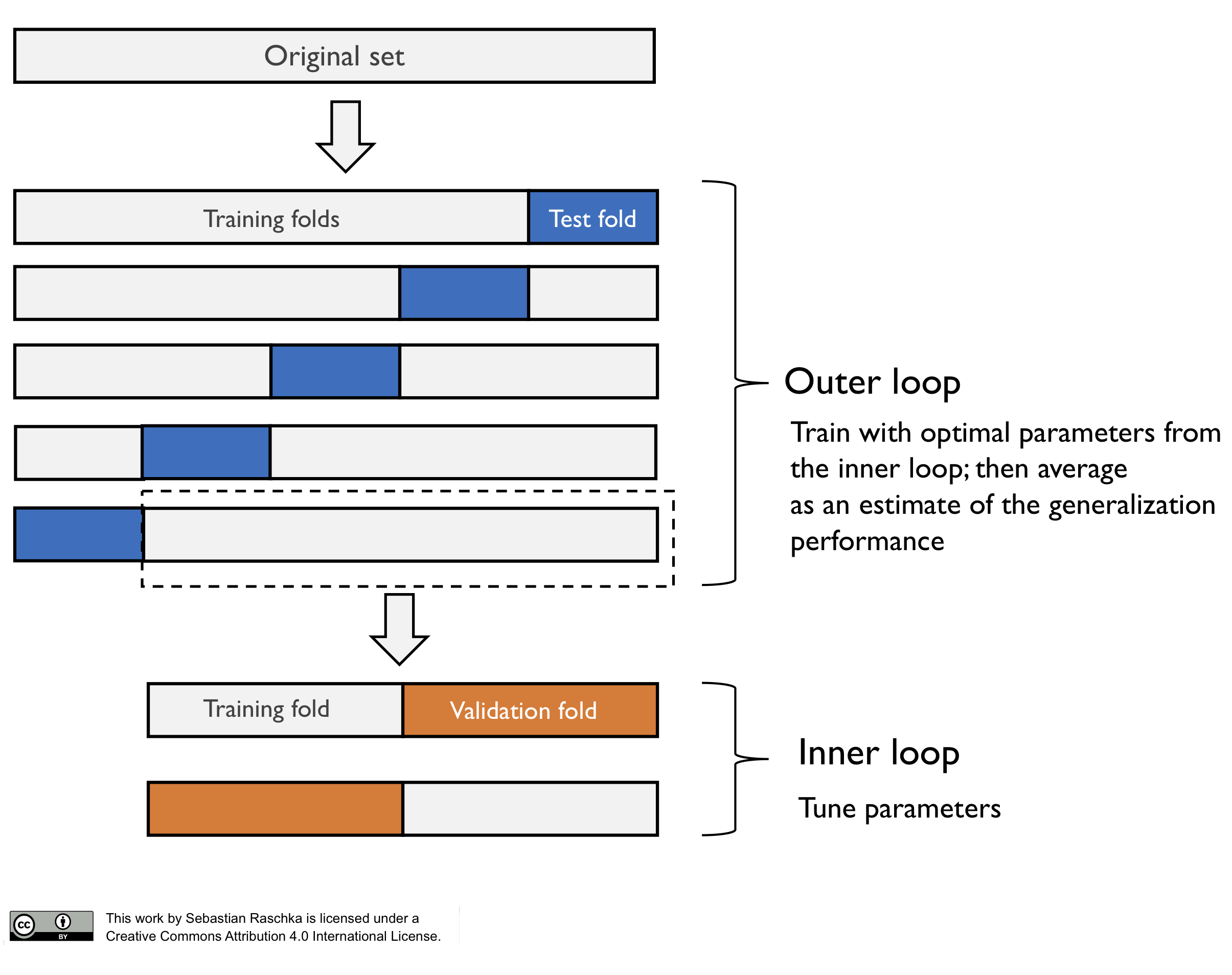
Note that in this particular case, this is a 5x2 setup (5-fold cross-validation in the outer loop, and 2-fold cross-validation in the inner loop). However, this is not the same as Dietterich’s 5x2cv method, which is an often confused scenario such that I want to highlight it here.
Code for using nested cross-validation with scikit-learn (Pedegrosa et al., 2011) can be found at https://github.com/rasbt/model-eval-article-supplementary/blob/master/code/nested_cv_code.ipynb.
Conclusions
Since “a picture is worth a thousand words,” I want to conclude this series on model evaluation, model selection, and algorithm selection with a figure (shown below) that summarizes my personal recommendations based on the concepts and literature that was reviewed.
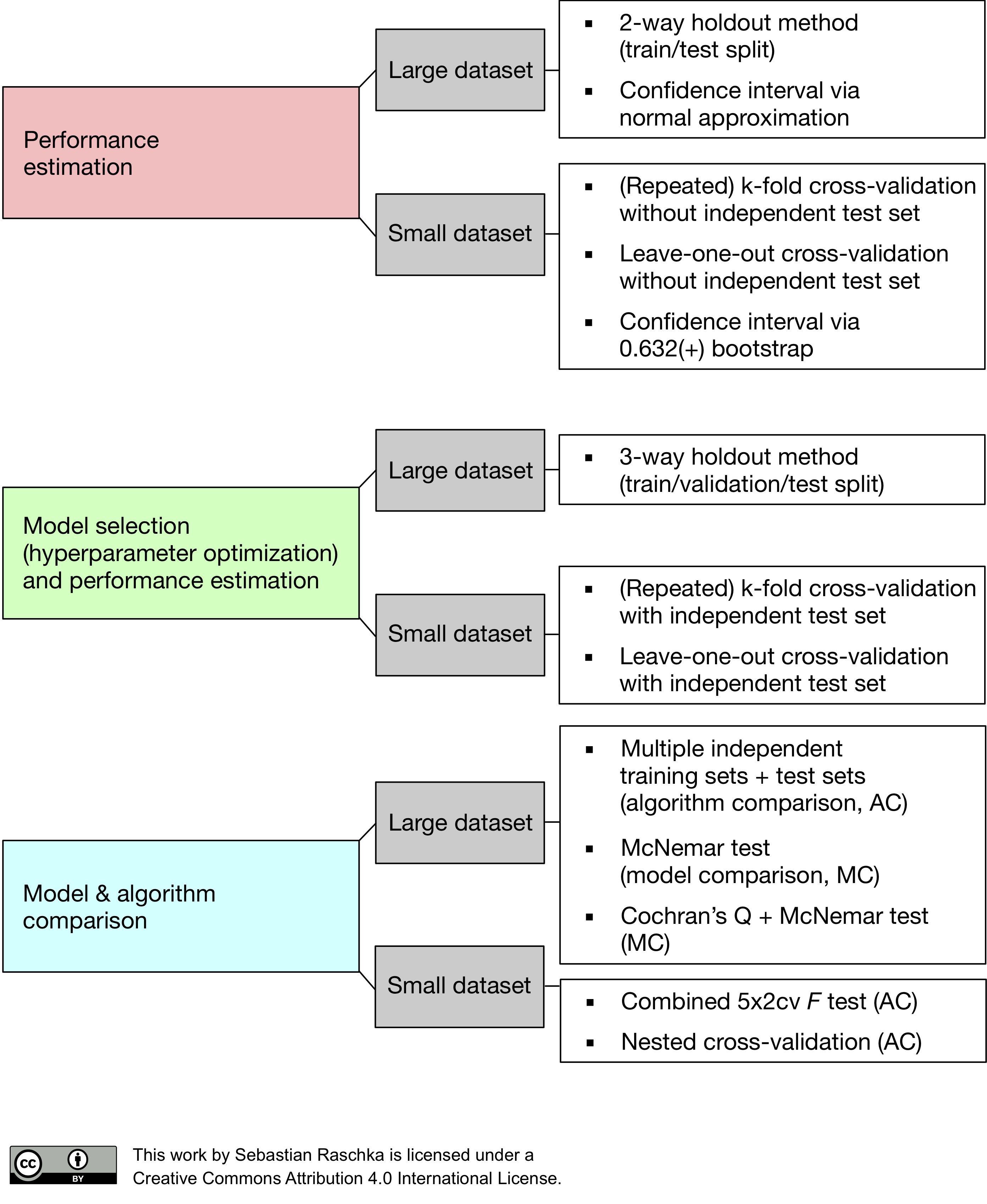
In this figure above, the abbreviation “MC” stands for “Model Comparison,” and “AC” stands for “Algorithm Comparison,” to distinguish these two tasks. It should be stressed that parametric tests for comparing model performances usually violate one or more independent assumptions (the models are not independent because the same training set was used, and the estimated generalization performances are not independent because the same test set was used.). In an ideal world, we would have access to the data generating distribution or at least an almost infinite pool of new data. However, in most practical applications, the size of the dataset is limited; hence, we can use one of the statistical tests discussed in this article as a heuristic to aid our decision making.
Note that the recommendations I listed in the figure above are suggestions and depend on the problem at hand. For instance, large test datasets (where “large” is relative but might refer to thousands or millions of data records), can provide reliable estimates of the generalization performance, whereas using a single training and test set when only a few data records are available can be problematic for several reasons discussed throughout Part II and Part III. If the dataset is very small, it might not be feasible to set aside data for testing, and in such cases, we can use k-fold cross-validation with a large k or Leave-one-out cross-validation as a workaround for evaluating the generalization performance. However, using these procedures, we have to bear in mind that we then do not compare between models but different algorithms that produce different models on the training folds. Nonetheless, the average performance over the different test folds can serve as an estimate for the generalization performance (Part III discussed the various implications for the bias and the variance of this estimate as a function of the number of folds).
For model comparisons, we usually do not have multiple independent test sets to evaluate the models on, so we can again resort to cross-validation procedures such as k-fold cross-validation, the 5x2cv method, or nested cross-validation. As Gael Varoquaux writes:
“Cross-validation is not a silver bullet. However, it is the best tool available, because it is the only non-parametric method to test for model generalization.” (Varoquaux, 2017)
As parting words, I hope you found this series of articles useful, and if you do have any questions or concerns, please do not hesitate to reach out – this is a blog article after all, which does not mean we cannot make adjustments :).
Thank you for reading. If you liked this content, you can also find me on Twitter, where I share more helpful content.
References
- Alpaydin, Ethem. “Combined 5x2 cv F test for comparing supervised classification learning algorithms.” Neural computation 11, no. 8 (1999): 1885-1892.
- Bonferroni, Carlo E. “Teoria statistica delle classi e calcolo delle probabilita.” Libreria internazionale Seeber, 1936.
- Cochran, William G. “The comparison of percentages in matched samples.” Biometrika 37, no. 3/4 (1950): 256-266.
- Dietterich, Thomas G. “Approximate statistical tests for comparing supervised classification learning algorithms.” Neural computation 10, no. 7 (1998): 1895-1923.
- Dunn, Olive Jean. “Multiple comparisons among means.” Journal of the American Statistical Association 56.293 (1961): 52-64.
- Edwards, Allen L. “Note on the “correction for continuity” in testing the significance of the difference between correlated proportions.” Psychometrika 13.3 (1948): 185-187.
- Fleiss, Joseph L., Bruce Levin, and Myunghee Cho Paik. Statistical methods for rates and proportions. John Wiley & Sons, 2013.
- Iizuka, Norio, Masaaki Oka, Hisafumi Yamada-Okabe, Minekatsu Nishida, Yoshitaka Maeda, Naohide Mori, Takashi Takao et al. “Oligonucleotide microarray for prediction of early intrahepatic recurrence of hepatocellular carcinoma after curative resection.” The Lancet 361, no. 9361 (2003): 923-929.
- Kuncheva, Ludmila I. Combining pattern classifiers: methods and algorithms. John Wiley & Sons, 2004.
- Looney, Stephen W. “A statistical technique for comparing the accuracies of several classifiers.” Pattern Recognition Letters8, no. 1 (1988): 5-9.
- McNemar, Quinn. “Note on the sampling error of the difference between correlated proportions or percentages.” Psychometrika 12.2 (1947): 153-157.
- Neyman, Jerzy, and Egon S. Pearson. “On the use and interpretation of certain test criteria for purposes of statistical inference: Part I.” Biometrika (1928): 175-240.
- Pedregosa, Fabian, Gaël Varoquaux, Alexandre Gramfort, Vincent Michel, Bertrand Thirion, Olivier Grisel, Mathieu Blondel, et al. “Scikit-learn: Machine learning in Python.” Journal of Machine Learning Research 12, no. Oct (2011): 2825-2830.
- Perneger, Thomas V. “What’s wrong with Bonferroni adjustments.” BMJ: British Medical Journal 316.7139 (1998): 1236.
- Raschka, Sebastian. “MLxtend: Providing machine learning and data science utilities and extensions to Python’s scientific computing stack.” The Journal of Open Source Software 3, no. 24 (2018).
- Rothman, Kenneth J. “No adjustments are needed for multiple comparisons.” Epidemiology 1.1 (1990): 43-46.
- Varma, Sudhir, and Richard Simon. “Bias in error estimation when using cross-validation for model selection.” BMC bioinformatics 7, no. 1 (2006): 91.
- Varoquaux, Gael. “Cross-validation failure: small sample sizes lead to large error bars.” Neuroimage (2017).
- Westfall, Peter H., James F. Troendle, and Gene Pennello. “Multiple McNemar tests.” Biometrics 66.4 (2010): 1185-1191.
This blog is personal passion project that does not offer direct compensation. However, for those who wish to support me, please consider purchasing a copy of one of my books. If you find them insightful and beneficial, please feel free to recommend them to your friends and colleagues.


Your support means a great deal! Thank you!