The Parzen-window method (also known as Parzen-Rosenblatt window method) is a widely used non-parametric approach to estimate a probability density function p(x) for a specific point p(x) from a sample p(x_n) that doesn’t require any knowledge or assumption about the underlying distribution.

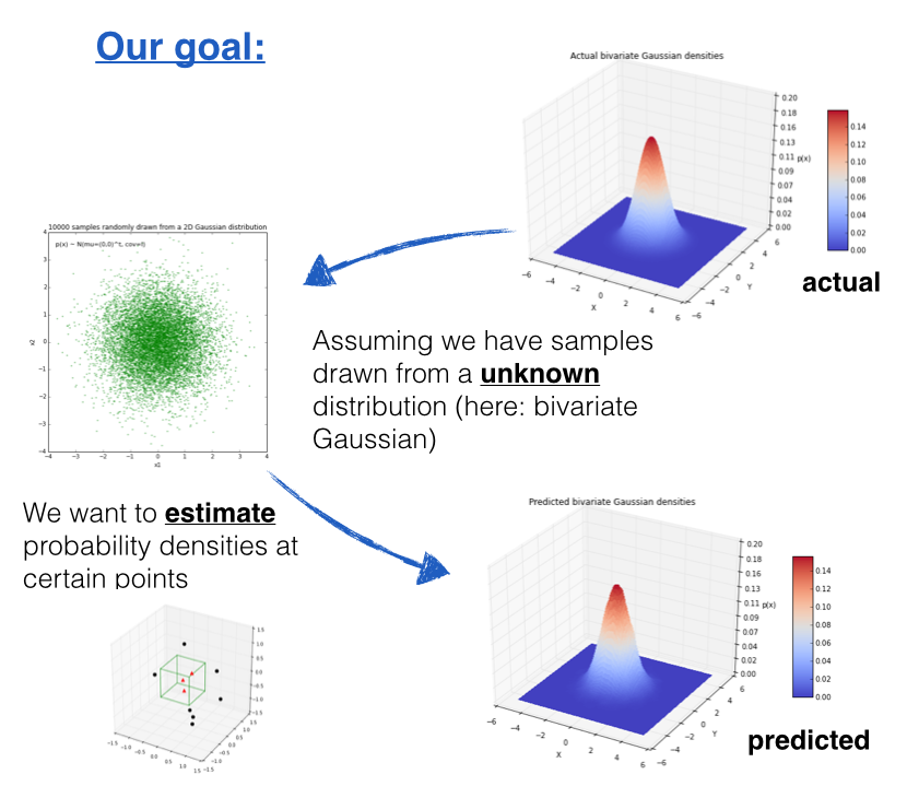
Table of Contents

• Table of Contents
• 1 Introduction
• 2 Defining the Region R_n
  • 2.1 Two different approaches - fixed volume vs. fixed number of samples in a variable volume
    • Case 1 - fixed volume:
    • Case 2 - fixed k:
  • 2.2 Example 3D-hypercubes
  • 2.3 The window function
    • 2.3.1 Implementing the window function
    • 2.3.2 Quantifying the sample points inside the 3D-hypercube
  • 2.4 Parzen-window estimation
  • 2.5 Critical assumption: Convergence
  • 2.6 Critical parameters of the Parzen-window technique: window width and kernel
  • 2.7 Implementing the Parzen-window estimation
• 3 Applying the Parzen-window approach to a random multivariate Gaussian dataset
  • 3.1 Generating 10000 random 2D-patterns from a Gaussian distribution
  • 3.2 Implementing and plotting the multivariate Gaussian density function
    • 3.2.1 Plotting the bivariate Gaussian densities
    • 3.2.2 Implementing the code to calculate the multivariate Gaussian densities
      • 3.2.2.1 Testing the multivariate Gaussian PDF implementation
    • 3.2.3 Comparing the Parzen-window estimation to the actual densities
      • 3.2.3.1 Choosing an appropriate window size
      • 3.2.3.2 Estimated vs. actual densities
      • 3.2.3.3 Plotting the estimated bivariate Gaussian densities
• 4 Conclusion and Drawbacks of the Parzen-window technique
• 5 Replacing the hypercube with a Gaussian Kernel
  • 5.1 Summarizing the implementation of the Parzen-window estimation with a hypercube kernel
    • 5.2 Using the Gaussian Kernel from scipy.stats
    • 5.3 Comparing Gaussian and hypercube kernel for a arbitrary window width
    • 5.4 Comparing the different bandwidth estimation calculations for the Gaussian kernel
• 6 Plotting the estimates from the different Kernels
  • 6.1 Window width effects: local peaks and averaging
• 7 Using the kernel density estimation for a pattern classification task
  • Bayes classifier
  • 7.1 Generating a sample training and test dataset
  • 7.2 Implementing the classifier using Bayes’ decision rule
  • 7.3 Density estimation via the Parzen-window technique with a Gaussian kernel
  • 7.4 Classifying the test data and calculating the error rate
  • Conclusion

1 Introduction

The Parzen-window method (also known as Parzen-Rosenblatt window method) is a widely used non-parametric approach to estimate a probability density function p(x) for a specific point p(x) from a sample p(x_n) that doesn’t require any knowledge or assumption about the underlying distribution.

Putting it in context - Where would this method be useful?

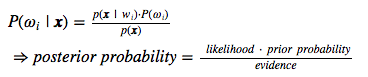
A popular application of the Parzen-window technique is to estimate the class-conditional densities (or also often called ‘likelihoods’) p(x | ω_i) in a supervised pattern classification problem from the training dataset (where p(x) refers to a multi-dimensional sample that belongs to particular class ω_i)).

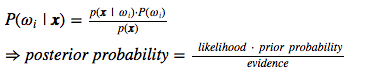
Imagine that we are about to design a Bayes classifier for solving a statistical pattern classification task using Bayes’ rule:

If the parameters of the the class-conditional densities (also called likelihoods) are known, it is pretty easy to design the classifier. I have solved some simple examples in IPython notebooks under the section Parametric Approaches.

About the mathematical notation:

Throughout this article, I will be adopting the common matrix notation that is used by most algebra textbooks:

• bold-face lowercase letter in italics (e.g., x) for vectors

• bold-face capital letter in italics (e.g., A) for matrices

• the subscripts to refer to elements by row and columns (e.g., \(A_{ij}\) for cell in row i and column j))

  ---

However, it becomes much more challenging, if we don’t don’t have prior knowledge about the underlying parameters that define the model of our data.

Imagine we are about to design a classifier for a pattern classification task where the parameters of the underlying sample distribution are not known. Therefore, we wouldn’t need the knowledge about the whole range of the distribution; it would be sufficient to know the probability of the particular point, which we want to classify, in order to make the decision. And here we are going to see how we can estimate this probability from the training sample.

However, the only problem of this approach would be that we would seldom have exact values - if we consider the histogram of the frequencies for a arbitrary training dataset. Therefore, we define a certain region (i.e., the Parzen-window) around the particular value to make the estimate.

And where does this name Parzen-window come from?

As it was quite common in the earlier days, this technique was named after its inventor, Emanuel Parzen, who published his detailed mathematical analysis in 1962 in the Annals of Mathematical Statistics [1]. About the same time, a second statistician, Murray Rosenblatt [2], discovered (or developed) this technique independently from Parzen so that the method is sometimes also referred to as Parzen-Rosenblatt window method.

[1] Parzen, Emanuel. On Estimation of a Probability Density Function and Mode. The Annals of Mathematical Statistics 33 (1962), no. 3, 1065–1076. doi:10.1214/aoms/1177704472.

[2] Rosenblatt, Murray. Remarks on Some Nonparametric Estimates of a Density Function. The Annals of Mathematical Statistics 27 (1956), no. 3, 832–837. doi:10.1214/aoms/1177728190.

2 Defining the Region R_n

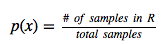
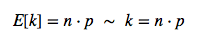
The basis of this approach is to count how many samples fall within a specified region \(R_{n}\) (or “window” if you will). Our intuition tells us, that (based on the observation), the probability that one sample falls into this region is

To tackle this problem from a more mathematical standpoint to estimate “the probability of observing k points out of n in a Region R “ we consider a binomial distribution

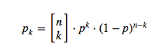
and make the assumption that in a binomial distribution, the probability peaks sharply at the mean, so that:

And if we think of the probability as a continuous variable, we know that it is defined as:

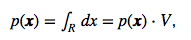
where V is the volume of the region R, and if we rearrange those terms, so that we arrive at the following equation, which we will use later:

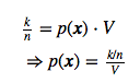
This simple equation above (i.e, the “probability estimate”) lets us calculate the probability density of a point x by counting how many points k fall in a defined region (or volume).

2.1 Two different approaches - fixed volume vs. fixed number of samples in a variable volume

Now, there are two possible approaches to estimate the densities at different points \(p(\mathbf{x})\).

Case 1 - fixed volume:

For a particular number n (= number of total points), we use volume V of a fixed size and observe how many points k fall into the region. In other words, we use the same volume to make an estimate at different regions.

The Parzen-window technique falls into this category!

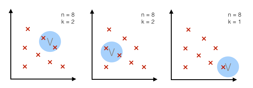
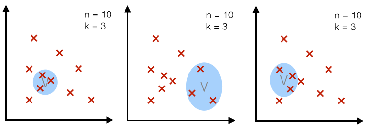
Case 2 - fixed k:

For a particular number n (= number of total points), we use a fixed number k (number of points that fall inside the region or volume) and adjust the volume accordingly. (The k-nearest neighbor technique uses this approach, which will be discussed in a separate article.)

2.2 Example 3D-hypercubes

To illustrate this with an example and a set of equations, let us assume this region R_n is a hypercube. And the volume of this hypercube is defined by V_n = h_n^d, where h_n is the length of the hypercube, and d is the number of dimensions.
For an 2D-hypercube with length 1, for example, this would be V₁ = 1² and for a 3D hypercube V_1 = 1³, respectively.

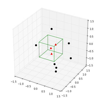
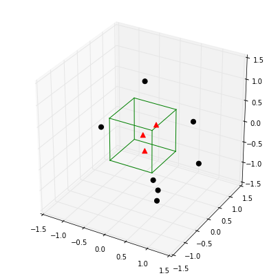
So let us visualize such a simple example: a typical 3-dimensional unit hypercube (h₁ = 1) representing the region R₁, and 10 sample points, where 3 of them lie within the hypercube (red triangles), and the other 7 outside (blue dots).

Note that using a hypercube would not be an ideal choice for a real application, but it certainly makes the implementations of the following steps a lot shorter and easier to follow.

%matplotlib inline

from mpl_toolkits.mplot3d import Axes3D
import matplotlib.pyplot as plt
import numpy as np
from itertools import product, combinations
fig = plt.figure(figsize=(7,7))
ax = fig.gca(projection='3d')
ax.set_aspect("equal")

# Plot Points

# samples within the cube
X_inside = np.array([[0,0,0],[0.2,0.2,0.2],[0.1, -0.1, -0.3]])

X_outside = np.array([[-1.2,0.3,-0.3],[0.8,-0.82,-0.9],[1, 0.6, -0.7],
                  [0.8,0.7,0.2],[0.7,-0.8,-0.45],[-0.3, 0.6, 0.9],
                  [0.7,-0.6,-0.8]])

for row in X_inside:
    ax.scatter(row[0], row[1], row[2], color="r", s=50, marker='^')

for row in X_outside:
    ax.scatter(row[0], row[1], row[2], color="k", s=50)

# Plot Cube
h = [-0.5, 0.5]
for s, e in combinations(np.array(list(product(h,h,h))), 2):
    if np.sum(np.abs(s-e)) == h[1]-h[0]:
        ax.plot3D(*zip(s,e), color="g")

ax.set_xlim(-1.5, 1.5)
ax.set_ylim(-1.5, 1.5)
ax.set_zlim(-1.5, 1.5)

plt.show()

2.3 The window function

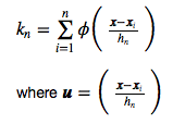
Once we visualized the region R₁ like above, it is easy and intuitive to count how many samples fall within this region, and how many lie outside. To approach this problem more mathematically, we would use the following equation to count the samples k_n within this hypercube, where φ is our so-called window function

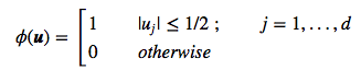
for a hypercube of unit length 1 centered at the coordinate system’s origin.

What this function basically does is assigning a value 1 to a sample point if it lies within 1/2 of the edges of the hypercube, and 0 if lies outside (note that the evaluation is done for all dimensions of the sample point).

If we extend on this concept, we can define a more general equation that applies to hypercubes of any length h_n that are centered at x:

2.3.1 Implementing the window function

def window_function(x_vec, unit_len=1):
"""
Implementation of the window function. Returns 1 if 3x1-sample vector
lies within a origin-centered hypercube, 0 otherwise.

"""
for row in x_vec:
    if np.abs(row) > (unit_len/2):
        return 0
return 1

2.3.2 Quantifying the sample points inside the 3D-hypercube

Using the window function that we just implemented above, let us now quantify how many points actually lie inside and outside the hypercube.

X_all = np.vstack((X_inside,X_outside))
assert(X_all.shape == (10,3))

k_n = 0
for row in X_all:
    k_n += window_function(row.reshape(3,1))

print('Points inside the hypercube:', k_n)
print('Points outside the hybercube:', len(X_all) - k_n)

Points inside the hypercube: 3
Points outside the hypercube: 7

2.4 Parzen-window estimation

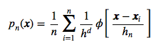
Based on the window function that we defined in the section above, we can now formulate the Parzen-window estimation with a hypercube kernel as follows:

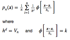
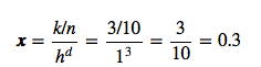
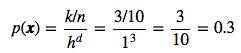
And applying this to our unit-hypercube example above, for which 3 out of 10 samples fall inside the hypercube (into region R), we can calculate the probability p(x) that x samples fall within region R as follows:

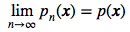
2.5 Critical assumption: Convergence

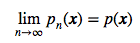
One of the most critical assumptions why the Parzen-window technique works (as well as the k-nearest neighbor technique) is that p_n (where the subscript n denotes the “number of samples”) converges to the true density p(x) when we assume an infinite number of training samples, which was nicely shown by Emanuel Parzen in his paper.

2.6 Critical parameters of the Parzen-window technique: window width and kernel

The two critical parameters in the Parzen-window techniques are

• 1) the window width
• 2) the kernel

1) window width:
Let us skip this part for now and discuss and explore the question of choosing an appropriate window width later by using an hands-on example.

2) kernel:
Most commonly, either a hypercube or a Gaussian kernel is used for the window function. But how do we know which is better? It really depends on the training sample. In practice, the choice is often made by testing the derived pattern classifier to see which method leads to a better performance on the test data set.
Intuitively, it would make sense to use a Gaussian kernel for a data set that follows a Gaussian distribution. But remember, the whole purpose of the Parzen-window estimation is to estimate densities of a unknown distribution! So, in practice we wouldn’t know whether our data stems from a Gaussian distribution or not (otherwise we wouldn’t need to estimate, but can use a parametric technique like MLE or Bayesian Estimation).
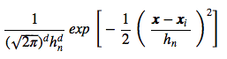
If we would decide to use a Gaussian kernel instead of the hypercube, we can just simply swap the terms of the window function, which we defined above for the hypercube, by:

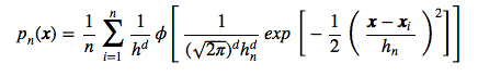
The Parzen-window estimation would then look like this:

mixing different kernels:
In some papers you will see, that the authors mixed hypercube and Gaussian kernels to estimate the densities at different regions. In practice, this might work very well, however, but note that in theory this would violate on of the underlying principles: that the density integrates to 1.

• A few other requirements are that at the limit the volume we choose for the Parzen-window becomes infinite small.

• The number of points k_n in this region converges to:

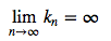
• from which we can conclude:

2.7 Implementing the Parzen-window estimation

And again, let us go to the more interesting part and implement the code for the hypercube kernel:

def parzen_window_est(x_samples, h=1, center=[0,0,0]):
    '''
    Implementation of the Parzen-window estimation for hypercubes.

    Keyword arguments:
        x_samples: A 'n x d'-dimensional numpy array, where each sample
            is stored in a separate row.
        h: The length of the hypercube.
        center: The coordinate center of the hypercube

    Returns the probability density for observing k samples inside the hypercube.

    '''
    dimensions = x_samples.shape[1]

    assert (len(center) == dimensions),  
            'Number of center coordinates have to match sample dimensions'
    k = 0
    for x in x_samples:
        is_inside = 1
        for axis,center_point in zip(x, center):
            if np.abs(axis-center_point) > (h/2):
                is_inside = 0
        k += is_inside
    return (k / len(x_samples)) / (h**dimensions)

print('p(x) =', parzen_window_est(X_all, h=1))

    p(x) = 0.3

At this point I can fully understand if you lost the overview a little bit. I summarized the three crucial parts (hypercube kernel, window function, and the resulting parzen-window estimation) in a later section, and I think it is worthwhile to take a brief look at it, before we apply it to a data set below.

3 Applying the Parzen-window approach to a random multivariate Gaussian dataset

Let us use an 2-dimensional dataset drawn from a multivariate Gaussian distribution to apply the Parzen-window technique for the density estimation.

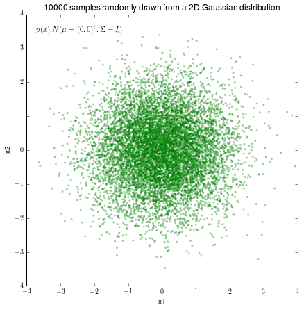
3.1 Generating 10000 random 2D-patterns from a Gaussian distribution

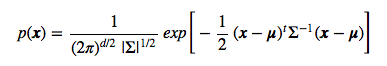
The general multivariate Gaussian probability density function (pdf) is defined as:

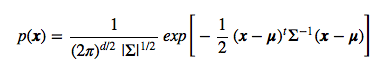
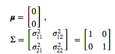
And we will use the following parameters for drawing the random samples:

import numpy as np

# Generate 10,000 random 2D-patterns
mu_vec = np.array([0,0])
cov_mat = np.array([[1,0],[0,1]])
x_2Dgauss = np.random.multivariate_normal(mu_vec, cov_mat, 10000)

print(x_2Dgauss.shape)

(10000, 2)

#from matplotlib import pyplot as plt

f, ax = plt.subplots(figsize=(7, 7))
ax.scatter(x_2Dgauss[:,0], x_2Dgauss[:,1],
        marker='o', color='green', s=4, alpha=0.3)
plt.title('10000 samples randomly drawn from a 2D Gaussian distribution')
plt.ylabel('x2')
plt.xlabel('x1')
ftext = 'p(x) ~ N(mu=(0,0)^t, cov=I)'
plt.figtext(.15,.85, ftext, fontsize=11, ha='left')
plt.ylim([-4,4])
plt.xlim([-4,4])

plt.show()

3.2 Implementing and plotting the multivariate Gaussian density function

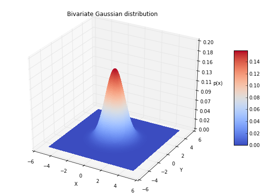
3.2.1 Plotting the bivariate Gaussian densities

First, let us plot the multivariate Gaussian distribution (here: bivariate) in a 3D plot to get an better idea of the actual density distribution.

#import numpy as np
#from matplotlib import pyplot as plt

from matplotlib.mlab import bivariate_normal
from mpl_toolkits.mplot3d import Axes3D

fig = plt.figure(figsize=(10, 7))
ax = fig.gca(projection='3d')
x = np.linspace(-5, 5, 200)
y = x
X,Y = np.meshgrid(x, y)
Z = bivariate_normal(X, Y)
surf = ax.plot_surface(X, Y, Z, rstride=1,
        cstride=1, cmap=plt.cm.coolwarm,
        linewidth=0, antialiased=False
    )

ax.set_zlim(0, 0.2)
ax.zaxis.set_major_locator(plt.LinearLocator(10))
ax.zaxis.set_major_formatter(plt.FormatStrFormatter('%.02f'))

ax.set_xlabel('X')
ax.set_ylabel('Y')
ax.set_zlabel('p(x)')

plt.title('Bivariate Gaussian distribution')
fig.colorbar(surf, shrink=0.5, aspect=7, cmap=plt.cm.coolwarm)

plt.show()

3.2.2 Implementing the code to calculate the multivariate Gaussian densities

To calculate the probabilities from the multivariate Gaussian density function and compare the results our estimate, let us implement it using the following equation:

Unfortunately, there is currently no Python library that provides this functionality. Good news is, that scipy.stats.multivariate_normal.pdf() will be implemented in the new release candidate of scipy (v. 0.14).

#import numpy as np

def pdf_multivariate_gauss(x, mu, cov):
    '''
    Caculate the multivariate normal density (pdf)

    Keyword arguments:
        x = numpy array of a "d x 1" sample vector
        mu = numpy array of a "d x 1" mean vector
        cov = "numpy array of a d x d" covariance matrix
    '''
    assert(mu.shape[0] > mu.shape[1]),\
        'mu must be a row vector'
    assert(x.shape[0] > x.shape[1]),\
        'x must be a row vector'
    assert(cov.shape[0] == cov.shape[1]),\
        'covariance matrix must be square'
    assert(mu.shape[0] == cov.shape[0]),\
        'cov_mat and mu_vec must have the same dimensions'
    assert(mu.shape[0] == x.shape[0]),\
        'mu and x must have the same dimensions'

    part1 = 1 / ( ((2* np.pi)**(len(mu)/2)) * (np.linalg.det(cov)**(1/2)) )
    part2 = (-1/2) * ((x-mu).T.dot(np.linalg.inv(cov))).dot((x-mu))
    return float(part1 * np.exp(part2))

3.2.2.1 Testing the multivariate Gaussian PDF implementation

Let us quickly confirm that the multivariate Gaussian, which we just implemented, works as expected by comparing it with the bivariate Gaussian from the matplotlib.mlab package.

from matplotlib.mlab import bivariate_normal

x = np.array([[0],[0]])
mu = np.array([[0],[0]])
cov = np.eye(2)

mlab_gauss = bivariate_normal(x,x)
mlab_gauss = float(mlab_gauss[0]) # because mlab returns an np.array
impl_gauss = pdf_multivariate_gauss(x, mu, cov)

print('mlab_gauss:', mlab_gauss)
print('impl_gauss:', impl_gauss)
assert(mlab_gauss == impl_gauss),\
        'Implementations of the mult. Gaussian return different pdfs'

mlab_gauss: 0.15915494309189535
impl_gauss: 0.15915494309189535

3.2.3 Comparing the Parzen-window estimation to the actual densities

And finally, let us compare the densities that we estimate using our implementation of the Parzen-window estimation with the actual multivariate Gaussian densities.

But before we do the comparison, we have to ask ourselves one more question: Which window size should we choose (i.e., what should be the side length h of our hypercube)? The window width is a function of the number of training samples,

But why √n, not just n?

This is because the number of k_n points within a window grows much smaller than the number of training samples, although

we have: k < n

This is also one of the biggest drawbacks of the Parzen-window technique, since in practice, the number of training data is usually (too) small, which makes the choice of an ‘optimal’ window size difficult.

In practice, one would choose different window widths and analyze which one results in the best performance of the derived classifier. The only guideline we have is that we assume that ‘optimal’ the window width shrinks with the number of training samples.

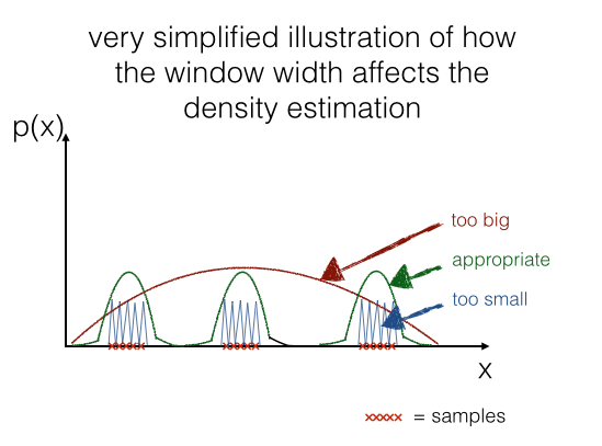
If we would choose a window width that is “too small”, this would result in local spikes, and a window width that is “too big” would average over the whole distribution. Below, I try to illustrate it using a 1D-sample.

In a later section we will have a look how it looks like in case of our example data data:

3.2.3.1 Choosing an appropriate window size

For our example, we have the luxury of knowing the distribution of our data, so let us look at some possible window widths to see how it affects the density estimation for the center of the distribution
(based on our test in the section above, we would expect a value close to p(x) = 0.1592 ).

print('Predict p(x) at the center [0,0]: ')

print('h = 0.1 ---> p(x) =', parzen_window_est(
        x_2Dgauss, h=0.1, center=[0, 0])
        )
print('h = 0.3 ---> p(x) =',parzen_window_est(
        x_2Dgauss, h=0.3, center=[0, 0])
        )
print('h = 0.6 ---> p(x) =',parzen_windo    w_est(
        x_2Dgauss, h=0.6, center=[0, 0])
        )
print('h = 1 ---> p(x) =',parzen_window_est(
        x_2Dgauss, h=1, center=[0, 0])
        )

Predict p(x) at the center [0,0]:
h = 0.1 ---> p(x) = 0.17999999999999997
h = 0.3 ---> p(x) = 0.1766666666666667
h = 0.6 ---> p(x) = 0.15694444444444444
h = 1 ---> p(x) = 0.1475

This rough estimate above gives us some idea about a window size that would give us a quite reasonable estimate: A good value for \(h\) should be somewhere around 0.6.

But we can do better (maybe I should use a minimization algorithm here, but I think this example should illustrate the procedure sufficiently). So let us create 400 evenly spaced values between (0,1) for h and see which gives us the estimate for the probability at the center of the distribution.

import operator

# generate a range of 400 window widths between 0 < h < 1
h_range = np.linspace(0.001, 1, 400)

# calculate the actual density at the center [0, 0]
mu = np.array([[0],[0]])
cov = np.eye(2)
actual_pdf_val = pdf_multivariate_gauss(np.array([[0],[0]]), mu, cov)

# get a list of the differnces (|estimate-actual|) for different window widths
parzen_estimates = [np.abs(parzen_window_est(x_2Dgauss, h=i, center=[0, 0])
               - actual_pdf_val) for i in h_range]

# get the window width for which |estimate-actual| is closest to 0
min_index, min_value = min(enumerate(parzen_estimates), key=operator.itemgetter(1))

print('Optimal window width for this data set: ', h_range[min_index])

Optimal window width for this data set:  0.554330827068

3.2.3.2 Estimated vs. actual densities

Now, that we have a “appropriate” window width, let us compare the estimates to the actual densities for some example points.

import prettytable

p1 = parzen_window_est(x_2Dgauss, h=h_range[min_index], center=[0, 0])
p2 = parzen_window_est(x_2Dgauss, h=h_range[min_index], center=[0.5, 0.5])
p3 = parzen_window_est(x_2Dgauss, h=h_range[min_index], center=[0.3, 0.2])

mu = np.array([[0],[0]])
cov = np.eye(2)

a1 = pdf_multivariate_gauss(np.array([[0],[0]]), mu, cov)
a2 = pdf_multivariate_gauss(np.array([[0.5],[0.5]]), mu, cov)
a3 = pdf_multivariate_gauss(np.array([[0.3],[0.2]]), mu, cov)

results = prettytable.PrettyTable(["", "predicted", "actual"])
results.add_row(["p([0,0]^t",p1, a1])
results.add_row(["p([0.5,0.5]^t",p2, a2])
results.add_row(["p([0.3,0.2]^t",p3, a3])

print(results)

+---------------+----------------+---------------------+
|               |   predicted    |        actual       |
+---------------+----------------+---------------------+
|   p([0,0]^t   | 0.159151557695 | 0.15915494309189535 |
| p([0.5,0.5]^t | 0.122208992134 | 0.12394999430965298 |
| p([0.3,0.2]^t | 0.150755520068 | 0.14913891880709737 |
+---------------+----------------+---------------------+

As we can see in the table above, our prediction works quite well!

3.2.3.3 Plotting the estimated bivariate Gaussian densities

Last but not least, let us plot the densities that we’d predict using the Parzen-window technique with a hypercube.

#import numpy as np
#from matplotlib import pyplot as plt
from mpl_toolkits.mplot3d import Axes3D

##############################################
### Predicted bivariate Gaussian densities ###
##############################################

fig = plt.figure(figsize=(10, 7))
ax = fig.gca(projection='3d')

X = np.linspace(-5, 5, 100)
Y = np.linspace(-5, 5, 100)
X,Y = np.meshgrid(X,Y)

Z = []
for i,j in zip(X.ravel(),Y.ravel()):
    Z.append(parzen_window_est(x_2Dgauss, h=h_range[min_index], center=[i, j]))

Z = np.asarray(Z).reshape(100,100)
surf = ax.plot_surface(X, Y, Z, rstride=1, cstride=1, cmap=plt.cm.coolwarm,
        linewidth=0, antialiased=False)

ax.set_zlim(0, 0.2)

ax.zaxis.set_major_locator(plt.LinearLocator(10))
ax.zaxis.set_major_formatter(plt.FormatStrFormatter('%.02f'))

ax.set_xlabel('X')
ax.set_ylabel('Y')
ax.set_zlabel('p(x)')

plt.title('Predicted bivariate Gaussian densities')

fig.colorbar(surf, shrink=0.5, aspect=7, cmap=plt.cm.coolwarm)

###########################################
### Actual bivariate Gaussian densities ###
###########################################

fig = plt.figure(figsize=(10, 7))
ax = fig.gca(projection='3d')
x = np.linspace(-5, 5, 100)
y = x
X,Y = np.meshgrid(x, y)
Z = bivariate_normal(X, Y)
surf = ax.plot_surface(X, Y, Z, rstride=1, cstride=1, cmap=plt.cm.coolwarm,
       linewidth=0, antialiased=False)

ax.set_zlim(0, 0.2)

ax.zaxis.set_major_locator(plt.LinearLocator(10))
ax.zaxis.set_major_formatter(plt.FormatStrFormatter('%.02f'))

fig.colorbar(surf, shrink=0.5, aspect=7, cmap=plt.cm.coolwarm)

ax.set_xlabel('X')
ax.set_ylabel('Y')
ax.set_zlabel('p(x)')

plt.title('Actual bivariate Gaussian densities')

plt.show()

4 Conclusion and Drawbacks of the Parzen-window technique

As we see in the two figures above (estimated vs. actual bivariate Gaussian probability distributions), we were able to estimate the Gaussian densities reasonably well.

Computation and performance

One of the biggest drawbacks of the Parzen-window technique is that we have to keep our training dataset around for estimating (computing) the probability densities. For example, if we design a Bayes’ classifier and use the Parzen-window technique to estimate the class-conditional probability densities p(x_i | ω_j), the computational task requires the whole training dataset to make the estimate for every point

• this is a disadvantage of non-parametric approaches in general.
  In contrast, parametric methods, e.g., the Maximum Likelihood Estimate (MLE) or Bayesian Estimation (BE) only require the training data to calculate the value of the parameters. Once, the parameters were obtained from the training dataset, it can be discarded and re-computation is not required for classifying data in the test dataset. However, in Bayesian Learning (BL), new samples can be incorporated to improve the estimated parameter values.

Size of the training data set

Since the Parzen-window technique estimates the probability densities based on the training dataset, it also relies on a reasonable size of training samples to make a “good” estimate. The more training samples we have in the the training dataset, roughly speaking, the more accurate the estimation becomes (Central limit theorem) since we reduce the likelihood of encountering a sparsity of points for local regions - assuming that our training samples are i.i.d (independently drawn and identically distributed). However, on the other hand, a larger number or training samples will also lead to a decrease of the computational performance as discussed in the section above.

Choosing the appropriate window width

Choosing an appropriate window width is a very challenging task, since we have no knowledge about the distribution of the training data (otherwise the non-parametric approach would be obsolete), and therefore we have to evaluate different window width by analyzing the performance of the derived classifier in a pattern classification task, using the assumption

as a guideline.

Choosing the kernel

Most commonly, either a hypercube or Gaussian kernel is chosen for the Parzen-window function φ. However, it is impossible to tell which kernel would yield a better estimation of the probability densities beforehand, since we assume that we don’t have any knowledge about the underlying distribution when we are using he Parzen-window technique. Similar to choosing an appropriate window width, we also have to evaluate the performance of the derived classifier to make a practical choice.

5 Replacing the hypercube with a Gaussian Kernel

Working through the examples above, we estimated the probability densities for a bivariate Gaussian distribution using a hypercube kernel, and our Parzen-window estimation was implemented by the following equation:

Now, let us switch to a Gaussian kernel for the Parzen-window estimation, so that the equation becomes:

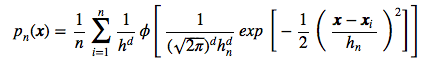
where

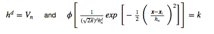
And applying this to out unit-hypercube example above, for which 3 out of 10 samples fall inside the hypercube (region R), we can calculate the probability p(x) that x samples fall within region R as follows:

5.1 Summarizing the implementation of the Parzen-window estimation with a hypercube kernel

Let us quickly summarize how we implemented the Parzen-window estimation for the hypercube.

def hypercube_kernel(h, x, x_i):
    """
    Implementation of a hypercube kernel for Parzen-window estimation.

    Keyword arguments:
        h: window width
        x: point x for density estimation, 'd x 1'-dimensional numpy array
        x_i: point from training sample, 'd x 1'-dimensional numpy array

    Returns a 'd x 1'-dimensional numpy array as input for a window function.

    """
    assert (x.shape == x_i.shape), 'vectors x and x_i must have the same dimensions'
    return (x - x_i) / (h)


def parzen_window_func(x_vec, h=1):
    """
    Implementation of the window function. Returns 1 if 'd x 1'-sample vector
    lies within inside the window, 0 otherwise.

    """
    for row in x_vec:
        if np.abs(row) > (1/2):
            return 0
    return 1


def parzen_estimation(x_samples, point_x, h, d, window_func, kernel_func):
    """
    Implementation of a parzen-window estimation.

    Keyword arguments:
        x_samples: A 'n x d'-dimensional numpy array, where each sample
            is stored in a separate row. (= training sample)
        point_x: point x for density estimation, 'd x 1'-dimensional numpy array
        h: window width
        d: dimensions
        window_func: a Parzen window function (phi)
        kernel_function: A hypercube or Gaussian kernel functions

    Returns the density estimate p(x).

    """
    k_n = 0
    for row in x_samples:
        x_i = kernel_func(h=h, x=point_x, x_i=row[:,np.newaxis])
        k_n += window_func(x_i, h=h)
    return (k_n / len(x_samples)) / (h**d)

Let’s go back to the hypercube example where 3 points lie inside, 7 points lie outside the hypercube, and our density estimate for a unit-1 hypercube at the center is p(x) = 0.3.

from mpl_toolkits.mplot3d import Axes3D
import matplotlib.pyplot as plt
import numpy as np
from itertools import product, combinations
fig = plt.figure(figsize=(7,7))
ax = fig.gca(projection='3d')
ax.set_aspect("equal")

# Plot Points

# samples within the cube
X_inside = np.array([[0,0,0],[0.2,0.2,0.2],[0.1, -0.1, -0.3]])

X_outside = np.array([[-1.2,0.3,-0.3],[0.8,-0.82,-0.9],[1, 0.6, -0.7],
                  [0.8,0.7,0.2],[0.7,-0.8,-0.45],[-0.3, 0.6, 0.9],
                  [0.7,-0.6,-0.8]])

for row in X_inside:
    ax.scatter(row[0], row[1], row[2], color="r", s=50, marker='^')

for row in X_outside:
    ax.scatter(row[0], row[1], row[2], color="k", s=50)

# Plot Cube
h = [-0.5, 0.5]
for s, e in combinations(np.array(list(product(h,h,h))), 2):
    if np.sum(np.abs(s-e)) == h[1]-h[0]:
        ax.plot3D(*zip(s,e), color="g")

ax.set_xlim(-1.5, 1.5)
ax.set_ylim(-1.5, 1.5)
ax.set_zlim(-1.5, 1.5)

plt.show()

We can now use the parzen_estimation() function with the hypercube kernel to calculate p(x).

point_x = np.array([[0],[0],[0]])

print('p(x) =', parzen_estimation(X_all, point_x, h=1, d=3,
                                 window_func=parzen_window_func,
                                 kernel_func=hypercube_kernel
                                 )
     )

p(x) = 0.3

And let us quickly confirm that it works on a bigger dataset for non-unit hypercubes that are not centered at the origin:
(Note that I just chose an arbitrary length for h, this is likely not the best choice for h.)

import numpy as np

# Generate 10000 random 2D-patterns
mu_vec = np.array([0,0])
cov_mat = np.array([[1,0],[0,1]])
x_2Dgauss = np.random.multivariate_normal(mu_vec, cov_mat, 10000)

import prettytable

p1 = parzen_estimation(x_2Dgauss, np.array([[0],[0]]), h=0.3, d=2,
                                 window_func=parzen_window_func,
                                 kernel_func=hypercube_kernel)
p2 = parzen_estimation(x_2Dgauss, np.array([[0.5],[0.5]]), h=0.3, d=2,
                                 window_func=parzen_window_func,
                                 kernel_func=hypercube_kernel)
p3 = parzen_estimation(x_2Dgauss, np.array([[0.3],[0.2]]), h=0.3, d=2,
                                 window_func=parzen_window_func,
                                 kernel_func=hypercube_kernel)

mu = np.array([[0],[0]])
cov = np.eye(2)

a1 = pdf_multivariate_gauss(np.array([[0],[0]]), mu, cov)
a2 = pdf_multivariate_gauss(np.array([[0.5],[0.5]]), mu, cov)
a3 = pdf_multivariate_gauss(np.array([[0.3],[0.2]]), mu, cov)

results = prettytable.PrettyTable(["", "p(x) predicted", "p(x) actual"])
results.add_row(["p([0,0]^t",p1, a1])
results.add_row(["p([0.5,0.5]^t",p2, a2])
results.add_row(["p([0.3,0.2]^t",p3, a3])

print(results)

+---------------+---------------------+---------------------+
|               |    p(x) predicted   |     p(x) actual     |
+---------------+---------------------+---------------------+
|   p([0,0]^t   |  0.1488888888888889 | 0.15915494309189535 |
| p([0.5,0.5]^t | 0.11777777777777779 | 0.12394999430965298 |
| p([0.3,0.2]^t |  0.1511111111111111 | 0.14913891880709737 |
+---------------+---------------------+---------------------+

5.2 Using the Gaussian Kernel from scipy.stats

Since we already went through the Parzen-window technique step by step for the hypercube kernel, let us import the gaussian_kde class from the scipy package for a more convenient approach.

The complete documentation can be found on docs.scipy.org.

The gaussian_kde class takes 2 parameters as input

• dataset : array_like Datapoints to estimate from. In case of univariate data this is a 1-D array, otherwise a 2-D array with shape (# of dims, # of data).

• bw_method : str, scalar or callable, optional The method used to calculate the estimator bandwidth. This can be 'scott', 'silverman', a scalar constant or a callable. If a scalar, this will be used directly as kde.factor. If a callable, it should take a gaussian_kde instance as only parameter and return a scalar. If 'None' (default), 'scott' is used. See Notes for more details.

Note initializiation of a gaussian_kde instance requires a numpy array in which the different samples are ordered by columns and where the rows reflect the dimensions of the dataset - this is why we have to pass our previously generated training data in its transposed form.

First have a quick look how the gaussian_kde() method works using a simple scalar as window width, like we did with the hypercube kernel before and estimate the density at the center.

# Example evaluating the density at the center

from scipy.stats import kde

density = kde.gaussian_kde(x_2Dgauss.T, bw_method=0.3)
print(density.evaluate(np.array([[0],[0]])))

[ 0.14652936]

5.3 Comparing Gaussian and hypercube kernel for a arbitrary window width

Let us now compare the Gaussian kernel against the hypercube for the same arbitrarily chosen window width:

import prettytable

gde = kde.gaussian_kde(x_2Dgauss.T, bw_method=0.3)

results = prettytable.PrettyTable(["", "p(x) hypercube kernel",
    "p(x) Gaussian kernel", "p(x) actual"])
results.add_row(["p([0,0]^t",p1, gde.evaluate(np.array([[0],[0]]))[0], a1])
results.add_row(["p([0.5,0.5]^t",p2, gde.evaluate(np.array([[0.5],[0.5]]))[0], a2])
results.add_row(["p([0.3,0.2]^t",p3, gde.evaluate(np.array([[0.3],[0.2]]))[0], a3])

print(results)

+---------------+-----------------------+----------------------+---------------------+
|               | p(x) hypercube kernel | p(x) Gaussian kernel |     p(x) actual     |
+---------------+-----------------------+----------------------+---------------------+
|   p([0,0]^t   |   0.1488888888888889  |    0.146529357818    | 0.15915494309189535 |
| p([0.5,0.5]^t |  0.11777777777777779  |    0.11282184148     | 0.12394999430965298 |
| p([0.3,0.2]^t |   0.1511111111111111  |    0.137350626774    | 0.14913891880709737 |
+---------------+-----------------------+----------------------+---------------------+

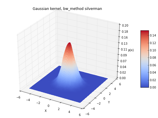
5.4 Comparing the different bandwidth estimation calculations for the Gaussian kernel

The gaussian_kde() class comes with 2 different “bandwith estimation calculations”, let us explore if it makes a difference to choose one over the other on our dataset:

from scipy.stats import kde
import prettytable

mu = np.array([[0],[0]])
cov = np.eye(2)

scott = kde.gaussian_kde(x_2Dgauss.T, bw_method='scott')
silverman = kde.gaussian_kde(x_2Dgauss.T, bw_method='silverman')
scalar = kde.gaussian_kde(x_2Dgauss.T, bw_method=0.3)
actual = pdf_multivariate_gauss(np.array([[0],[0]]), mu, cov)

results = prettytable.PrettyTable(["", "p([0,0]^t gaussian kernel"])
results.add_row(["bw_method scalar 0.3:", scalar.evaluate(np.array([[0],[0]]))[0]])
results.add_row(["bw_method scott:", scott.evaluate(np.array([[0],[0]]))[0]])
results.add_row(["bw_method silverman:", silverman.evaluate(np.array([[0],[0]]))[0]])
results.add_row(["actual density:", actual])

print(results)

+-----------------------+---------------------------+
|                       | p([0,0]^t gaussian kernel |
+-----------------------+---------------------------+
| bw_method scalar 0.3: |       0.146529357818      |
|    bw_method scott:   |       0.153502928635      |
|  bw_method silverman: |       0.153502928635      |
|    actual density:    |    0.15915494309189535    |
+-----------------------+---------------------------+

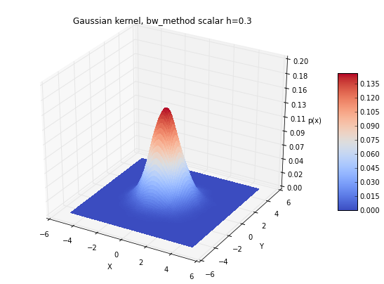
6 Plotting the estimates from the different Kernels

And eventually, let us plot the results for the different Gaussian kernel bandwidth estimation methods for the estimated distribution.

import numpy as np
from matplotlib import pyplot as plt
from matplotlib.mlab import bivariate_normal
from mpl_toolkits.mplot3d import Axes3D

X = np.linspace(-5, 5, 100)
Y = np.linspace(-5, 5, 100)
X,Y = np.meshgrid(X,Y)


##########################################
### Hypercube kernel density estimates ###
##########################################

fig = plt.figure(figsize=(10, 7))
ax = fig.gca(projection='3d')

Z = []
for i,j in zip(X.ravel(),Y.ravel()):
    Z.append(parzen_estimation(x_2Dgauss, np.array([[i],[j]]), h=0.3, d=2,
                                 window_func=parzen_window_func,
                                 kernel_func=hypercube_kernel))

Z = np.asarray(Z).reshape(100,100)
surf = ax.plot_surface(X, Y, Z, rstride=1, cstride=1, cmap=plt.cm.coolwarm,
        linewidth=0, antialiased=False)

ax.set_zlim(0, 0.2)

ax.zaxis.set_major_locator(plt.LinearLocator(10))
ax.zaxis.set_major_formatter(plt.FormatStrFormatter('%.02f'))

ax.set_xlabel('X')
ax.set_ylabel('Y')
ax.set_zlabel('p(x)')

plt.title('Hypercube kernel with window width h=0.3')

fig.colorbar(surf, shrink=0.5, aspect=7, cmap=plt.cm.coolwarm)

plt.show()

#########################################
### Gaussian kernel density estimates ###
#########################################

for bwmethod,t in zip([scalar, scott, silverman], ['scalar h=0.3', 'scott',
        'silverman']):
    fig = plt.figure(figsize=(10, 7))
    ax = fig.gca(projection='3d')
    Z = bwmethod(np.array([X.ravel(),Y.ravel()]))
    Z = Z.reshape(100,100)
    surf = ax.plot_surface(X, Y, Z, rstride=1, cstride=1, cmap=plt.cm.coolwarm,
        linewidth=0, antialiased=False)

    ax.set_zlim(0, 0.2)
    ax.zaxis.set_major_locator(plt.LinearLocator(10))
    ax.zaxis.set_major_formatter(plt.FormatStrFormatter('%.02f'))
    ax.set_xlabel('X')
    ax.set_ylabel('Y')
    ax.set_zlabel('p(x)')

    plt.title('Gaussian kernel, bw_method %s' %t)
    fig.colorbar(surf, shrink=0.5, aspect=7, cmap=plt.cm.coolwarm)
    plt.show()



###########################################
### Actual bivariate Gaussian densities ###
###########################################


fig = plt.figure(figsize=(10, 7))
ax = fig.gca(projection='3d')
Z = bivariate_normal(X, Y)
surf = ax.plot_surface(X, Y, Z, rstride=1, cstride=1, cmap=plt.cm.coolwarm,
        linewidth=0, antialiased=False)

ax.set_zlim(0, 0.2)

ax.zaxis.set_major_locator(plt.LinearLocator(10))
ax.zaxis.set_major_formatter(plt.FormatStrFormatter('%.02f'))
fig.colorbar(surf, shrink=0.5, aspect=7, cmap=plt.cm.coolwarm)

ax.set_xlabel('X')
ax.set_ylabel('Y')
ax.set_zlabel('p(x)')
plt.title('Actual bivariate Gaussian densities')

plt.show()

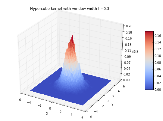
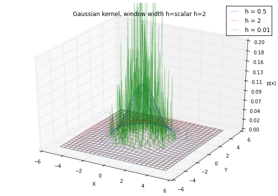
6.1 Window width effects: local peaks and averaging

As we have discussed in an earlier section, choosing an appropriate window width can be a challenging task, if we choose a window width that is too small, we will end up with local spikes in the densities, and if we choose a window width that is too large, we will be averaging over the entire distribution:

gde_01 = kde.gaussian_kde(x_2Dgauss.T, bw_method=0.01)
gde_5 = kde.gaussian_kde(x_2Dgauss.T, bw_method=0.5)
gde_20 = kde.gaussian_kde(x_2Dgauss.T, bw_method=2)

for bwmethod,t in zip([gde_01, gde_5, gde_20],
        ['scalar h=0.05', 'scalar h=0.5', 'scalar h=2']):
    fig = plt.figure(figsize=(10, 7))
    ax = fig.gca(projection='3d')
    Z = bwmethod(np.array([X.ravel(),Y.ravel()]))
    Z = Z.reshape(100,100)
    surf = ax.plot_surface(X, Y, Z, rstride=1, cstride=1, cmap=plt.cm.coolwarm,
        linewidth=0, antialiased=False)

    ax.set_zlim(0, 0.2)
    ax.zaxis.set_major_locator(plt.LinearLocator(10))
    ax.zaxis.set_major_formatter(plt.FormatStrFormatter('%.02f'))
    ax.set_xlabel('X')
    ax.set_ylabel('Y')
    ax.set_zlabel('p(x)')

    plt.title('Gaussian kernel, window width h=%s' %t)
    fig.colorbar(surf, shrink=0.5, aspect=7, cmap=plt.cm.coolwarm)
    plt.show()

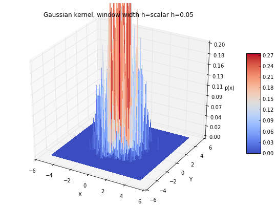
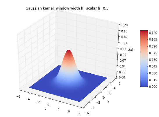
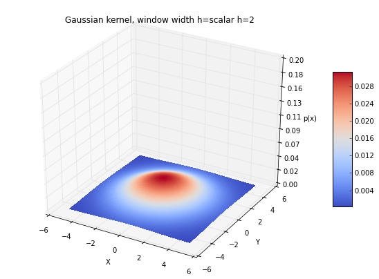
fig = plt.figure(figsize=(10, 7))
ax = fig.gca(projection='3d')

Z = gde_5(np.array([X.ravel(),Y.ravel()]))
Z = Z.reshape(100,100)
surf = ax.plot_wireframe(X, Y, Z, rstride=4, cstride=4,
    alpha=0.3, label='h = 0.5')

Z = gde_20(np.array([X.ravel(),Y.ravel()]))
Z = Z.reshape(100,100)
surf = ax.plot_wireframe(X, Y, Z, color='red',
    rstride=4, cstride=4, alpha=0.3, label='h = 2')

Z = gde_01(np.array([X.ravel(),Y.ravel()]))
Z = Z.reshape(100,100)
surf = ax.plot_wireframe(X, Y, Z, color='green',
    rstride=4, cstride=4, alpha=0.3, label='h = 0.01')
ax.set_zlim(0, 0.2)
ax.zaxis.set_major_locator(plt.LinearLocator(10))
ax.zaxis.set_major_formatter(plt.FormatStrFormatter('%.02f'))
ax.set_xlabel('X')
ax.set_ylabel('Y')
ax.set_zlabel('p(x)')
ax.legend()

plt.title('Gaussian kernel, window width h=%s' %title)

plt.show()

7 Using the kernel density estimation for a pattern classification task

In the introduction I mentioned that a popular application of the Parzen-window technique is to estimate the class-conditional densities (or also often called ‘likelihoods’) p(x* | ω)* in a supervised pattern classification problem from the training dataset (where x is a multi-dimensional sample that belongs to particular class ω_i).
Now, let us use the kernel density estimation for designing a simple Bayes-classifier.

Bayes’ Rule

To design a minimum error classifier, we will use Bayes’ rule:

Decision Rule

Where the posterior probability is used to define our decision rule. E.g., for a simple 2-class problem with the two class labels ω₁ and ω₂:

decide ω₁ if P(ω₁ | *x ) > P(ω₂ | x ), else decide *ω₂

Objective function

For this example, let us simplify the problem a little bit. We will assume that we have equal prior probabilities (the probability to encounter a particular class is equal):
P(ω₁ | *x )* = P(ω₂ | *x )* = … = P(ω₁ | *x )* = 1/n

And since p(x) is just a scale factor that is equal for all posterior probabilities, we can drop it from the equation.

Now, we can simplify the decision rule, so that it just depends on the priors. For a 2-class problem, this would be

decide ω₁ if P(ω₁ | *x ) > P(ω₂ | x ), else decide *ω₂

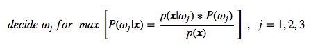
Bayes classifier

And in more general (for multiple classes), our classifier becomes
ω_j -> max[P(ω₁ | *x )] for *j = 1, 2, …, c

7.1 Generating a sample training and test dataset

Let us generate random 2-dimensional data for 3 classes from a multivariate Gaussian distribution with the following parameters:

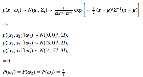
Now, we will create 120 random samples for each of the 3 classes, and divide it into a equally-sized training and test data set, so that each set will contain 30 samples from each class.

import numpy as np

# Covariance matrices
cov_mats = {}
for i in range(1,4):
    cov_mats[i] = i * np.eye(2)

# mean vectors    
mu_vecs = {}
for i,j in zip(range(1,4), [[0,0], [3,0], [4,5]]):
    mu_vecs[i] = np.array(j).reshape(2,1)

# Example for accessing parameters, e.g., mu_vec and cov_mat for class2
print('mu_vec2\n', mu_vecs[2])
print('cov_mat2\n', cov_mats[2])

mu_vec2
 [[3]
 [0]]
cov_mat2
 [[ 2.  0.]
 [ 0.  2.]]

# Generating the random samples
all_samples = {}
for i in range(1,4):
    # generating 40x2 dimensional arrays with random Gaussian-distributed samples
    class_samples = np.random.multivariate_normal(mu_vecs[i].ravel(), cov_mats[i], 40)
    # adding class label to 3rd column
    class_samples = np.append(class_samples, np.zeros((40,1))+i, axis=1)
    all_samples[i] = class_samples

# Dividing the samples into training and test datasets
train_set = np.append(all_samples[1][0:20], all_samples[2][0:20], axis=0)
train_set = np.append(train_set, all_samples[3][0:20], axis=0)

test_set = np.append(all_samples[1][20:40], all_samples[2][20:40], axis=0)
test_set = np.append(test_set, all_samples[3][20:40], axis=0)

assert(train_set.shape == (60, 3))
assert(test_set.shape == (60, 3))

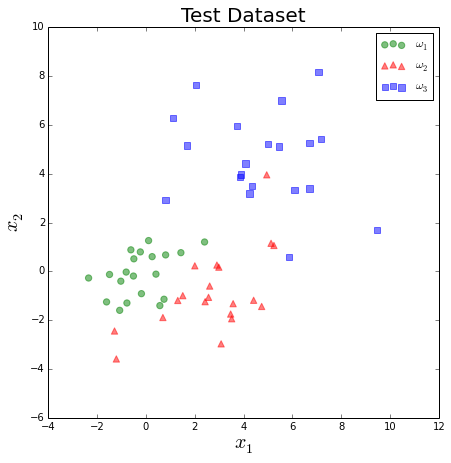
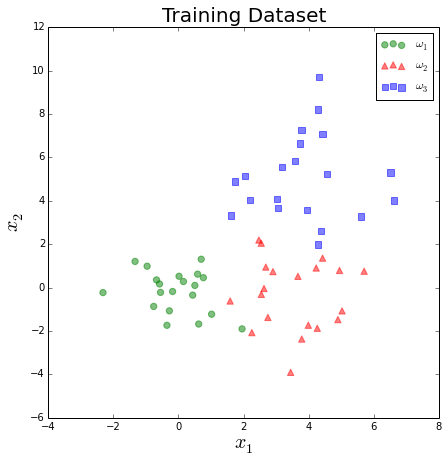
# Visualizing samples by plotting them in a scatter plot

import numpy as np
from matplotlib import pyplot as plt

for dset,title in zip((test_set, train_set), ['Test', 'Training']):
    f, ax = plt.subplots(figsize=(7, 7))
    ax.scatter(dset[dset[:,2] == 1][:,0], dset[dset[:,2] == 1][:,1], \
           marker='o', color='green', s=40, alpha=0.5, label='$\omega_1$')
    ax.scatter(dset[dset[:,2] == 2][:,0], dset[dset[:,2] == 2][:,1], \
           marker='^', color='red', s=40, alpha=0.5, label='$\omega_2$')
    ax.scatter(dset[dset[:,2] == 3][:,0], dset[dset[:,2] == 3][:,1], \
           marker='s', color='blue', s=40, alpha=0.5, label='$\omega_3$')
    plt.legend(loc='upper right')
    plt.title('{} Dataset'.format(title), size=20)
    plt.ylabel('$x_2$', size=20)
    plt.xlabel('$x_1$', size=20)
plt.show()

7.2 Implementing the classifier using Bayes’ decision rule

Now, let us implement the classifier. To recapitulate:

We can remove the prior probabilities (equal priors) and the scale factor:

import operator

def bayes_classifier(x_vec, kdes):
    """
    Classifies an input sample into class w_j determined by
    maximizing the class conditional probability for p(x|w_j).

    Keyword arguments:
        x_vec: A dx1 dimensional numpy array representing the sample.
        kdes: List of the gausssian_kde (kernel density) estimates

    Returns a tuple ( p(x|w_j)_value, class label ).

    """
    p_vals = []
    for kde in kdes:
        p_vals.append(kde.evaluate(x_vec))
    max_index, max_value = max(enumerate(p_vals), key=operator.itemgetter(1))
    return (max_value, max_index + 1)

7.3 Density estimation via the Parzen-window technique with a Gaussian kernel

or our convenience, let us use the scipy.stats library class kde for the kernel density estimation:

from scipy.stats import kde
class1_kde = kde.gaussian_kde(train_set[train_set[:,2] == 1].T[0:2],
        bw_method='scott')
class2_kde = kde.gaussian_kde(train_set[train_set[:,2] == 2].T[0:2],
        bw_method='scott')
class3_kde = kde.gaussian_kde(train_set[train_set[:,2] == 3].T[0:2],
        bw_method='scott')

7.4 Classifying the test data and calculating the error rate

Now, it is time to classify the test data and calculate the empirical error.

def empirical_error(data_set, classes, classifier_func, classifier_func_args):
    """
    Keyword arguments:
        data_set: 'n x d'- dimensional numpy array, class label in the last column.
        classes: List of the class labels.
        classifier_func: Function that returns the max argument from the discriminant function.
            evaluation and the class label as a tuple.
        classifier_func_args: List of arguments for the 'classifier_func'.
    
    Returns a tuple, consisting of a dictionary withthe classif. counts and the error.
    
    e.g., ( {1: {1: 321, 2: 5}, 2: {1: 0, 2: 317}}, 0.05)
    where keys are class labels, and values are sub-dicts counting for which class (key)
    how many samples where classified as such.
    
    """
    class_dict = {i:{j:0 for j in classes} for i in classes}

    for cl in classes:
        for row in data_set[data_set[:,-1] == cl][:,:-1]:
            g = classifier_func(row, *classifier_func_args)
            class_dict[cl][g[1]] += 1
    
    correct = 0
    for i in classes:
        correct += class_dict[i][i]
    
    misclass = data_set.shape[0] - correct
    return (class_dict, misclass / data_set.shape[0])

import prettytable

classification_dict, error = empirical_error(test_set, [1,2,3], bayes_classifier,
        [[class1_kde, class2_kde, class3_kde]])

labels_predicted = ['w{} (predicted)'.format(i) for i in [1,2,3]]
labels_predicted.insert(0,'test dataset')

train_conf_mat = prettytable.PrettyTable(labels_predicted)
for i in [1,2,3]:
    a, b, c = [classification_dict[i][j] for j in [1,2,3]]
    # workaround to unpack (since Python does not support just '*a')
    train_conf_mat.add_row(['w{} (actual)'.format(i), a, b, c])
print(train_conf_mat)
print('Empirical Error: {:.2f} ({:.2f}%)'.format(error, error * 100))

+--------------+----------------+----------------+----------------+
| test dataset | w1 (predicted) | w2 (predicted) | w3 (predicted) |
+--------------+----------------+----------------+----------------+
| w1 (actual)  |       19       |       1        |       0        |
| w2 (actual)  |       5        |       14       |       1        |
| w3 (actual)  |       0        |       1        |       19       |
+--------------+----------------+----------------+----------------+
Empirical Error: 0.13 (13.33%)

Conclusion

Given that we have a fairly small training sample size (20 samples per class), the error rate is fairly small on the test dataset. Given the convergence principle

We would likely improve the performance of the classifier if we would be able to increase the size of the training dataset. By the way, the performance on the training data set here is expected to be much better, since this is the data set used to derive the parameters.

classification_dict, error = empirical_error(train_set,
        [1,2,3], bayes_classifier, [[class1_kde, class2_kde, class3_kde]])

labels_predicted = ['w{} (predicted)'.format(i) for i in [1,2,3]]
labels_predicted.insert(0,'training dataset')

train_conf_mat = prettytable.PrettyTable(labels_predicted)
for i in [1,2,3]:
    a, b, c = [classification_dict[i][j] for j in [1,2,3]]
    # workaround to unpack (since Python does not support just '*a')
    train_conf_mat.add_row(['w{} (actual)'.format(i), a, b, c])
print(train_conf_mat)
print('Empirical Error: {:.2f} ({:.2f}%)'.format(error, error * 100))

  +------------------+----------------+----------------+----------------+
  | training dataset | w1 (predicted) | w2 (predicted) | w3 (predicted) |
  +------------------+----------------+----------------+----------------+
  |   w1 (actual)    |       20       |       0        |       0        |
  |   w2 (actual)    |       0        |       20       |       0        |
  |   w3 (actual)    |       0        |       1        |       19       |
  +------------------+----------------+----------------+----------------+
  Empirical Error: 0.02 (1.67%)